
Census API Python Tutorial: Regional Analysis Guide
Learn the Census API with Python. Download ACS data, compare U.S. regions, states and counties, handle FIPS codes, build maps, and create a regional notebook.
Census API Python Tutorial: Regional Analysis Guide
Method note: Main examples use the 2024 ACS 5 year Data Profiles and preserve official estimate and margin of error pairs.
The Census Data API lets you request U.S. Census Bureau statistics with a web address instead of downloading a large file by hand. In Python, the basic pattern is simple. You choose a year and dataset, ask for a small set of variables, choose a geography, send the request, and load the returned data into pandas.
This Census API Python Tutorial uses the 2024 American Community Survey 5 year Data Profiles as the main example. That release combines data collected from 2020 through 2024. The goal is practical: pull regional and state data, keep geography codes safe, work with margins of error, validate the result, and create charts that can be reproduced later.
A current Census API key is required for data queries. The Census Bureau also limits a standard query to 50 variables. The code below keeps the key in an environment variable called CENSUS_API_KEY, so it is not exposed in a notebook, screenshot, or shared repository.
Working example
import os
import requests
import pandas as pd

BASE_URL = "https://api.census.gov/data/2024/acs/acs5/profile"

variables = [
    "NAME",
    "DP05_0001E",
    "DP05_0001M",
    "DP03_0062E",
    "DP03_0062M",
    "DP03_0128PE",
    "DP03_0128PM",
    "DP02_0068PE",
    "DP02_0068PM",
]

api_key = os.getenv("CENSUS_API_KEY")
if not api_key:
    raise RuntimeError("Set CENSUS_API_KEY before running this request.")

params = {
    "get": ",".join(variables),
    "for": "region:*",
    "key": api_key,
}

response = requests.get(BASE_URL, params=params, timeout=30)
response.raise_for_status()
rows = response.json()

regions = pd.DataFrame(rows[1:], columns=rows[0])
print(regions.head())
In this guide
- Start With Census Data and Choose the Right Source
- Set Up Python, API Access, and a Safe Project
- Read a Census Request Before You Write Code
- Pull ACS Data Into pandas and Clean It Correctly
- Work With Regions, States, Counties, and Census Geography
- Build a Reusable Regional Analysis Workflow
- Compare U.S. Regions and Visualize the Results
- Validate, Troubleshoot, Document, and Reproduce the Analysis
Start With Census Data and Choose the Right Source
The first choice is not Python. It is the Census product. The Census Bureau publishes many programs, and the same topic can appear in more than one table or release. A good workflow starts by deciding what question you are asking, which geography you need, and how current the estimate must be.
What the Census Data API does
The Census Data API is a public data service for Census Bureau statistical datasets. You send a request that names a vintage, a dataset, one or more variables, and a geography. The service returns a simple response that Python can read. This is useful when you need the same query for many states, counties, or years, or when you want a process that can be repeated later.
The statistical API returns data values, not detailed map shapes. Census geography services such as TIGERweb provide boundaries when you need to draw a map. Keeping these roles separate helps avoid a common beginner mistake: expecting one API endpoint to provide both statistics and polygons.
ACS, Decennial Census, and PUMS
The American Community Survey, usually called the ACS, provides recurring estimates about people, households, housing, income, education, work, and many other topics. The Decennial Census is designed to count the population every ten years and is the better source for core population counts tied to a census year. PUMS provides individual level sample records with privacy protections. PUMS is powerful for custom analysis, but it is not the easiest starting point for a regional tutorial.
Table 1. Choosing among common Census products
| Product | Best use | Time coverage | Geography notes |
|---|---|---|---|
| ACS 1 year | Recent social and economic estimates for larger geographies | One year of survey data | Fewer small geographies are published than in the 5 year product |
| ACS 5 year | Broad geographic coverage and stable local estimates | Sixty months of survey data | Includes small geographies and is the main product used in this guide |
| Decennial Census | Core population and housing counts for a census year | Once every ten years | Strong choice for official census year counts |
| PUMS | Custom analysis using privacy protected person and housing records | Depends on the ACS PUMS release | Uses larger public use areas rather than every small geography |
This tutorial uses the 2024 ACS 5 year Data Profiles. The 2024 5 year release combines survey information collected from 2020 through 2024. Data Profiles are convenient because they put useful social, economic, housing, and demographic measures into a compact set of variables. Detailed Tables are better when you need very specific counts. Comparison Profiles are useful when change over time is the main question.
Set Up Python, API Access, and a Safe Project
You only need three Python packages for the core workflow: requests for the web request, pandas for cleaning and tables, and matplotlib for charts. A virtual environment keeps the project dependencies separate from other Python work.
python -m venv .venv

# Windows PowerShell
.venv\Scripts\Activate.ps1

# macOS or Linux
source .venv/bin/activate

pip install requests pandas matplotlib
Store the API key outside your code
Current Census documentation requires an API key for data queries. Registration is free. Treat the key like a project credential. Do not paste a real key into a public notebook, a screenshot, a Git repository, or an article sample.
# Windows PowerShell
$env:CENSUS_API_KEY="YOUR_KEY_HERE"

# macOS or Linux
export CENSUS_API_KEY="YOUR_KEY_HERE"
The Python examples read the key with os.getenv. If the variable is missing, the code stops with a clear message. This is safer than letting a request fail later with a vague response.
Use a small project structure
census_project/
    analysis.ipynb
    data/
        raw/
        clean/
    figures/
    notes/
Keep raw responses separate from cleaned tables when the project grows. Save figures in their own folder and record the dataset, vintage, variables, and retrieval date in a note or metadata file. A simple structure is enough. The goal is to make the work easy to repeat.
Read a Census Request Before You Write Code
A Census request is easier to debug when you can read it as a sentence. The base path identifies the year and dataset. The get parameter names the variables. The for parameter chooses the geography. The in parameter adds a parent geography when needed. The key parameter authenticates the data request.
https://api.census.gov/data/2024/acs/acs5/profile
?get=NAME,DP03_0062E,DP03_0062M
&for=region:*
&key=YOUR_KEY_HERE
Table 2. Main parts of a Census API request
| Part | Example | Meaning |
|---|---|---|
| Vintage | 2024 | The reference year for the dataset |
| Dataset | acs/acs5/profile | ACS 5 year Data Profiles |
| get | NAME,DP03_0062E | Variables returned in the response |
| for | region:* | All Census regions |
| in | state:06 | Parent geography used for a county request |
| key | Environment variable value | Required API credential |
Variables, labels, attributes, and group calls
A variable is a named field in a Census dataset. Some names are readable, while ACS variables often use codes such as DP03_0062E. Always open the variable page for the exact year and dataset you plan to use. A code from an older article may still exist, but you should not assume the definition stayed the same.
The get function tells the API which fields to return. Required variables are fields a particular dataset may need for a valid request. Attributes can provide related information such as annotations or margins of error. The descriptive parameter can add labels to output in supported queries. A group call can request all variables from a table group, but a beginner should start with a small list so the result stays easy to inspect.
Predicates and geography filters
The for and in parts are geography predicates. A wildcard selects all available values at that level. For example, region:* asks for every Census region, while county:* with in=state:06 asks for every county in California. The newer ucgid option can describe geography with a fully qualified geographic identifier. It is useful for more advanced cases, but for and in are easier to learn first.
Estimate and margin of error suffixes
Data Profile variable suffixes matter. E is commonly used for an estimate and M for its margin of error. PE represents a percentage estimate and PM represents the matching percentage margin of error. Pair the estimate and uncertainty fields before analysis so they stay together through cleaning and plotting.
Table 3. Variables used in the regional tutorial
| Variable | Readable name | Type | Matching uncertainty |
|---|---|---|---|
| DP05_0001E | Total population | Estimate | DP05_0001M |
| DP03_0062E | Median household income | Estimate | DP03_0062M |
| DP03_0128PE | People below the poverty level | Percent estimate | DP03_0128PM |
| DP02_0068PE | Bachelor degree or higher, age 25 and over | Percent estimate | DP02_0068PM |
The 2024 variable metadata identifies DP03_0062E as median household income in 2024 inflation adjusted dollars. It identifies DP03_0128PE as the percent of all people below the poverty level, and DP02_0068PE as the percent of people age 25 and over with a bachelor degree or higher. Those definitions are why the exact variable page belongs in the research notes.
JSON and CSV responses
JSON is a natural choice for Python because requests can decode it directly. The Census response is often a list of lists. The first row contains column names and the remaining rows contain data. CSV is useful when a file based workflow is more convenient. The analysis steps are similar once the data are in a DataFrame.
Pull ACS Data Into pandas and Clean It Correctly
Start with a small request that you can inspect. The regional example below asks for four regions and nine fields, including the geography name and four estimate and margin of error pairs. This is enough to prove that the request, key, variable codes, and geography all work before you build a larger pipeline.
First working request
import os
import requests
import pandas as pd

BASE_URL = "https://api.census.gov/data/2024/acs/acs5/profile"

variables = [
    "NAME",
    "DP05_0001E",
    "DP05_0001M",
    "DP03_0062E",
    "DP03_0062M",
    "DP03_0128PE",
    "DP03_0128PM",
    "DP02_0068PE",
    "DP02_0068PM",
]

api_key = os.getenv("CENSUS_API_KEY")
if not api_key:
    raise RuntimeError("Set CENSUS_API_KEY before running this request.")

params = {
    "get": ",".join(variables),
    "for": "region:*",
    "key": api_key,
}

response = requests.get(BASE_URL, params=params, timeout=30)
response.raise_for_status()
rows = response.json()

regions = pd.DataFrame(rows[1:], columns=rows[0])
print(regions.head())
requests.get sends the query parameters safely and builds the final URL. The timeout prevents a stalled connection from hanging forever. response.raise_for_status raises an exception for an unsuccessful HTTP response. response.json converts the JSON body into normal Python objects. The first returned row becomes the DataFrame column names.
Rename variables and convert measurements
rename_map = {
    "NAME": "region_name",
    "DP05_0001E": "population",
    "DP05_0001M": "population_moe",
    "DP03_0062E": "median_household_income",
    "DP03_0062M": "median_household_income_moe",
    "DP03_0128PE": "poverty_rate",
    "DP03_0128PM": "poverty_rate_moe",
    "DP02_0068PE": "bachelor_or_higher_rate",
    "DP02_0068PM": "bachelor_or_higher_rate_moe",
}

regions = regions.rename(columns=rename_map)

numeric_columns = [
    "population",
    "population_moe",
    "median_household_income",
    "median_household_income_moe",
    "poverty_rate",
    "poverty_rate_moe",
    "bachelor_or_higher_rate",
    "bachelor_or_higher_rate_moe",
]

for column in numeric_columns:
    regions[column] = pd.to_numeric(regions[column], errors="coerce")

regions["region"] = regions["region"].astype("string")

print(regions.dtypes)
print(regions)
Census API values often arrive as text. Convert measurement columns to numeric values before calculations. Keep geography identifiers as strings. A state FIPS code such as 06 must remain 06, not the number 6, or it will fail to join cleanly with other Census files.
Do not turn missing values into zero without evidence
A missing value and a real zero do not mean the same thing. Census responses can also include annotation fields or special values that need review. Use numeric conversion with errors set to coerce, inspect the resulting missing values, and check the metadata before deciding how to handle them. Replacing every missing value with zero can create a false result that looks valid.
Keep the raw response when the analysis matters
For a research or production project, save the original API response or a raw table before heavy transformation. If a result later looks odd, you can compare the cleaned table with the source response. This simple habit makes debugging much easier.
Work With Regions, States, Counties, and Census Geography
Census geography is hierarchical. Regions contain divisions, divisions contain states, and states contain counties. Smaller levels continue through places, county subdivisions, tracts, block groups, and other geography types. The exact levels supported depend on the dataset.
Four Census regions
The United States is divided into four Census regions: Northeast, Midwest, South, and West. In the 2024 ACS 5 year Data Profiles examples, region is geography level 020. A request with for=region:* returns the four region rows directly. This matters for medians. A regional median household income should come from the region geography when the dataset supports it. Do not average state medians and call that number the regional median.
State and county FIPS codes
State FIPS codes use two digits. County codes use three digits within a state. Joining them produces a five digit county GEOID. Keep all of these codes as strings so leading zeros survive.
county_variables = ["NAME", "DP05_0001E"]

params = {
    "get": ",".join(county_variables),
    "for": "county:*",
    "in": "state:06",
    "key": os.getenv("CENSUS_API_KEY"),
}

response = requests.get(BASE_URL, params=params, timeout=30)
response.raise_for_status()
rows = response.json()

counties = pd.DataFrame(rows[1:], columns=rows[0])
counties["state"] = counties["state"].astype("string").str.zfill(2)
counties["county"] = counties["county"].astype("string").str.zfill(3)
counties["GEOID"] = counties["state"] + counties["county"]

print(counties[["NAME", "state", "county", "GEOID"]].head())
In the example, California has state FIPS 06. A county code such as 001 becomes a five digit GEOID when it is combined with the state code. This pattern is the basis for joining statistical data to many Census boundary files.
When to use ucgid
The Census Data API user guide also documents ucgid as an alternative geography predicate. It can be useful when you already have fully qualified Census geographic identifiers or need geography variants that are awkward to express with for and in. For ordinary state and county tutorials, the older syntax is still easier to read.
Statistics and map shapes come from different services
The Data API provides statistical values. TIGERweb and TIGER boundary files provide geographic shapes. If you build a choropleth map, join the data and boundary table using the correct GEOID or FIPS fields. Do not use a state name as the only join key when a stable code is available.
Build a Reusable Regional Analysis Workflow
Copying a long requests block for every geography works once, but it becomes fragile quickly. A small helper function can centralize the key check, the 50 variable limit, URL construction, error handling, and DataFrame conversion.
Reusable census_get function
import os
import requests
import pandas as pd


def census_get(year, dataset, variables, for_clause, in_clause=None):
    api_key = os.getenv("CENSUS_API_KEY")
    if not api_key:
        raise RuntimeError("Set CENSUS_API_KEY before running a Census query.")

    if not variables:
        raise ValueError("Pass at least one variable.")

    if len(variables) > 50:
        raise ValueError("A standard Census API query supports up to 50 variables.")

    url = f"https://api.census.gov/data/{year}/{dataset}"
    params = {
        "get": ",".join(variables),
        "for": for_clause,
        "key": api_key,
    }

    if in_clause:
        params["in"] = in_clause

    response = requests.get(url, params=params, timeout=30)
    response.raise_for_status()
    rows = response.json()

    if not rows:
        return pd.DataFrame()

    if len(rows) == 1:
        return pd.DataFrame(columns=rows[0])

    return pd.DataFrame(rows[1:], columns=rows[0])
The function keeps the moving parts visible. You still pass the exact year, dataset, variables, and geography. That is helpful for reproducibility because the call itself documents what was requested.
Use the same function for regions, states, and counties
variables = [
    "NAME",
    "DP05_0001E",
    "DP05_0001M",
    "DP03_0062E",
    "DP03_0062M",
    "DP03_0128PE",
    "DP03_0128PM",
    "DP02_0068PE",
    "DP02_0068PM",
]

regions = census_get(
    year=2024,
    dataset="acs/acs5/profile",
    variables=variables,
    for_clause="region:*",
)

states = census_get(
    year=2024,
    dataset="acs/acs5/profile",
    variables=["NAME", "DP03_0062E", "DP03_0128PE"],
    for_clause="state:*",
)

california_counties = census_get(
    year=2024,
    dataset="acs/acs5/profile",
    variables=["NAME", "DP05_0001E"],
    for_clause="county:*",
    in_clause="state:06",
)
The region request is useful for regional medians and percentages. The state request supports a state level scatter plot. The county example shows a parent geography. The same function can be reused for other supported levels once you confirm the geography syntax on the official examples page.
Optional storage and pipeline tools
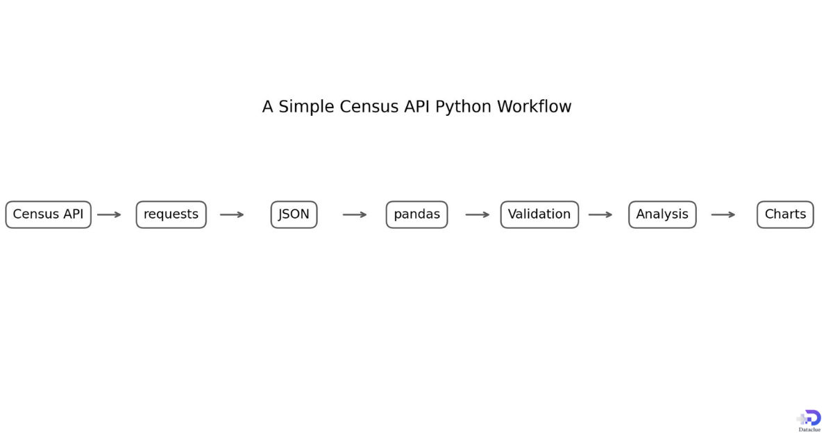
pandas is enough for this tutorial. If the project grows, you can load cleaned results into DuckDB, PostgreSQL, BigQuery, or another database. Pipeline tools such as dlt can help with repeated loads and schema management. Add that layer only after the direct API request is clear and tested. A pipeline should reduce repeated work, not hide how the Census request works.
Save clean results and metadata
from pathlib import Path
from datetime import date

output_dir = Path("data/clean")
output_dir.mkdir(parents=True, exist_ok=True)

regions.to_csv(
    output_dir / "acs_2024_5year_regions.csv",
    index=False,
)

metadata = {
    "vintage": 2024,
    "dataset": "acs/acs5/profile",
    "geography": "region:*",
    "retrieval_date": date.today().isoformat(),
    "variables": variables,
}

print(metadata)
A useful saved dataset should travel with enough metadata to rebuild it. Record the vintage, dataset path, variable list, geography, retrieval date, and important cleaning steps. If the analysis becomes part of a report, also save the code version that created the final table and figures.
Compare U.S. Regions and Visualize the Results
Regional analysis becomes more useful when you compare several measures rather than ranking one number. Population gives scale. Median household income and poverty describe different parts of economic conditions. Educational attainment adds another dimension. Margins of error remind you that ACS values are estimates, not exact counts for every measure.
Regional results from the 2024 ACS 5 year period
The static values below are 2024 ACS 5 year estimates that were cross checked against published summaries citing the U.S. Census Bureau. The API code in this tutorial retrieves the official estimate and margin of error fields directly when a valid key is supplied. To avoid publishing invented uncertainty values, the static table does not fill in margin of error numbers that were not retrieved in this writing environment.
Table 4. Regional snapshot from the 2024 ACS 5 year period
| Region | Population | Median household income | Poverty rate | Bachelor degree or higher |
|---|---|---|---|---|
| Northeast | 57,414,970 | $88,896 | 11.7% | 40.5% |
| Midwest | 69,108,736 | $75,973 | 12.0% | 33.8% |
| South | 129,288,316 | $74,552 | 13.6% | 33.8% |
| West | 79,110,477 | $91,752 | 11.6% | 36.8% |
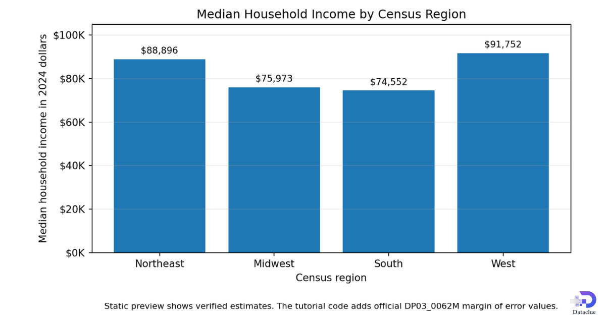
The South is the largest region by population in this snapshot. The West has the highest median household income among the four regions, followed by the Northeast. The South has the highest poverty rate in the table. The Northeast has the highest share of adults age 25 and over with a bachelor degree or higher. These are descriptive comparisons. They do not explain why the regions differ.
Plot median household income with margins of error
The visible preview below shows the verified median estimates. The publishing code that follows uses DP03_0062M as y error, so a reader with a Census API key can reproduce the full figure with official 90 percent ACS margins of error. Keeping the estimate and margin field together is more reliable than typing uncertainty values into a chart by hand.
import matplotlib.pyplot as plt
from matplotlib.ticker import FuncFormatter

plot_df = regions.sort_values("region")

fig, ax = plt.subplots(figsize=(8, 5))
ax.bar(
    plot_df["region_name"],
    plot_df["median_household_income"],
    yerr=plot_df["median_household_income_moe"],
    capsize=5,
)
ax.set_title("Median Household Income by Census Region")
ax.set_xlabel("Census region")
ax.set_ylabel("Median household income in 2024 dollars")
ax.set_ylim(bottom=0)
ax.yaxis.set_major_formatter(
    FuncFormatter(lambda value, position: f"${value / 1000:.0f}K")
)
ax.grid(axis="y", alpha=0.25)
fig.tight_layout()
plt.show()
If two confidence ranges overlap, do not automatically claim that one region is definitively higher than another. Overlap is not a complete statistical test, but it is a useful warning that a simple ranking may overstate precision. For a formal comparison, use the appropriate ACS significance testing guidance.
Look beyond a regional ranking with a state scatter plot
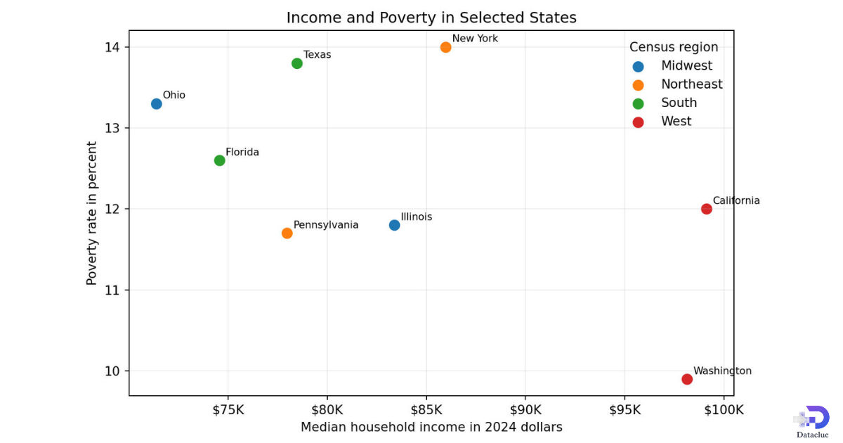
A scatter plot can show whether states with higher median household income also tend to have lower poverty rates. The static preview uses two selected states from each region so labels stay readable. The full Python code retrieves all states, maps their FIPS codes to Census regions, and plots the complete set.
region_by_state = {
    "09": "Northeast", "23": "Northeast", "25": "Northeast",
    "33": "Northeast", "44": "Northeast", "50": "Northeast",
    "34": "Northeast", "36": "Northeast", "42": "Northeast",
    "17": "Midwest", "18": "Midwest", "26": "Midwest",
    "39": "Midwest", "55": "Midwest", "19": "Midwest",
    "20": "Midwest", "27": "Midwest", "29": "Midwest",
    "31": "Midwest", "38": "Midwest", "46": "Midwest",
    "10": "South", "11": "South", "12": "South", "13": "South",
    "24": "South", "37": "South", "45": "South", "51": "South",
    "54": "South", "01": "South", "21": "South", "28": "South",
    "47": "South", "05": "South", "22": "South", "40": "South",
    "48": "South", "04": "West", "08": "West", "16": "West",
    "30": "West", "32": "West", "35": "West", "49": "West",
    "56": "West", "02": "West", "06": "West", "15": "West",
    "41": "West", "53": "West",
}

states = states.rename(columns={
    "NAME": "state_name",
    "DP03_0062E": "median_household_income",
    "DP03_0128PE": "poverty_rate",
})

states["state"] = states["state"].astype("string").str.zfill(2)
states["median_household_income"] = pd.to_numeric(
    states["median_household_income"], errors="coerce"
)
states["poverty_rate"] = pd.to_numeric(
    states["poverty_rate"], errors="coerce"
)
states["census_region"] = states["state"].map(region_by_state)

states = states.dropna(
    subset=["median_household_income", "poverty_rate", "census_region"]
)

fig, ax = plt.subplots(figsize=(8, 5))
for region, group in states.groupby("census_region"):
    ax.scatter(
        group["median_household_income"],
        group["poverty_rate"],
        label=region,
        alpha=0.8,
    )

ax.set_title("State Income and Poverty by Census Region")
ax.set_xlabel("Median household income in 2024 dollars")
ax.set_ylabel("Poverty rate in percent")
ax.legend(title="Census region", frameon=False)
ax.grid(alpha=0.2)
fig.tight_layout()
plt.show()
The scatter should be read as a pattern, not as proof of cause. Income and poverty are related to many factors, including cost of living, age, labor markets, household structure, and local policy. A useful chart helps you ask a better next question. It should not turn a correlation into a causal claim.
Optional map
A state choropleth can add geographic context when location is central to the question. Pull the statistic with the Census Data API, obtain state shapes from TIGERweb or a Census boundary file, join on the state GEOID, and label the source and vintage. Skip the map if a ranked bar chart answers the question more clearly.
Validate, Troubleshoot, Document, and Reproduce the Analysis
A Census script is not finished when it returns a DataFrame. It is finished when you have checked that the rows, codes, units, missing values, and variable definitions match the question you meant to ask.
Run basic validation checks
expected_regions = {"1", "2", "3", "4"}
actual_regions = set(regions["region"].dropna())

if actual_regions != expected_regions:
    raise ValueError(f"Unexpected region codes: {actual_regions}")

if regions["region"].duplicated().any():
    raise ValueError("Duplicate region rows found.")

if (regions["population"] <= 0).any():
    raise ValueError("Population must be positive.")

if not regions["poverty_rate"].between(0, 100).all():
    raise ValueError("Poverty rate must be between 0 and 100.")

if not regions["bachelor_or_higher_rate"].between(0, 100).all():
    raise ValueError("Education rate must be between 0 and 100.")

print("Validation checks passed.")
For state data, check that state codes have two characters after padding. For counties, check three digit county codes and five digit GEOIDs. Look for duplicate geographies. Confirm that percentages fall between 0 and 100. Check that the expected number of geography rows was returned. These tests catch many silent mistakes before they reach a chart.
Common Census API problems
Table 5. Common problems and practical fixes
| Problem | Likely cause | What to check |
|---|---|---|
| Missing or invalid key | CENSUS_API_KEY is empty or wrong | Print only whether the environment variable exists. Never print the real key in shared output |
| Invalid variable | Variable code does not exist in that vintage or dataset | Open the official variable page for the exact year and dataset |
| Geography error | The dataset does not support the requested for and in combination | Use the dataset geography page and examples |
| Too many variables | The query exceeds the standard 50 variable limit | Split the variables into smaller groups and merge on geography codes |
| Empty DataFrame | The request returned only a header or an unexpected response | Inspect response text, parameters, geography, and required variables |
| Lost leading zeros | FIPS codes were converted to numbers | Read and store geography codes as strings, then use zfill where appropriate |
| Strange missing values | Special values or annotations are present | Review metadata and annotation fields before replacing values |
Be careful when comparing ACS periods
ACS 5 year estimates are rolling periods. Two nearby releases can share several years of survey data. Geography boundaries can also change, and dollar measures can be expressed in different inflation adjusted years. Before calling a change a trend, check the period overlap, geography consistency, variable definition, margin of error, and dollar basis.
Reproducibility checklist
- Record the Census vintage and full dataset path.
- Save the exact variable codes and readable definitions.
- Record the geography query and any FIPS mapping used.
- Keep FIPS and GEOID values as strings.
- Save the retrieval date and the code version used for the final output.
- Keep estimate and margin of error fields paired.
- Document any rows you remove and any missing values you change.
- Use direct region estimates for regional medians when they are available.
Frequently asked questions
How do I specify different levels of "geography" or regions in the Census API?
for and inpredicates: {'for': 'state:*'}{'for': 'county:*', 'in': 'state:48'} (where 48 is the FIPS code for Texas){'for': 'tract:*', 'in': 'state:27 county:053'} &ucgid= predicate allows you to pull specific, non-contiguous multi-geographies simultaneously by passing exact GeoID strings. Do I need an API key for regional data analysis?
config.py file or a .env file and import it securely. [Which Census datasets should I use for regional profiling?
What are the best Python libraries for handling Census API data?
requests + pandas: The traditional stack. Use requests.get() to pull the JSON data from the API endpoint and convert the list of lists into a clean pd.DataFrame.pytidycensus: A Python equivalent to R's popular tidycensus package. It automatically formats API payloads directly into structural DataFrames and supports spatial data components. pygris & geopandas: Crucial for regional mapping. pygris downloads the official TIGER/Line shapefiles from the Census Bureau as GeoDataFrames, making it easy to create choropleth map visualizations.censusdis: A flexible, Pythonic package built to discover, load, and compute diversity and segregation metrics over various regional bounds. Why are my demographic numbers loading as text, and how do I calculate regional metrics?
Before conducting regional aggregation, you must parse the strings to integers or floats:
Do I need a Census API key for this Python tutorial?
Yes. Current Census documentation requires an API key for data queries. Store it in CENSUS_API_KEY rather than placing the real key inside the script.
Why use ACS 5 year data for regional analysis?
The 5 year product offers broad geography coverage and combines sixty months of survey data. It is also useful when the same workflow may later be extended to smaller geographies.
Can I average state median incomes to get a regional median?
No. A median is not additive. Query the region geography directly when the dataset provides the regional median.
Why are FIPS codes stored as text?
Codes such as California 06 contain leading zeros. Numeric conversion can remove those zeros and break joins.
What does an ACS margin of error mean?
It describes sampling uncertainty around an estimate at the stated confidence level used by the ACS. Keep it with the estimate and use it when judging how precise a comparison is.
When should I use TIGERweb?
Use TIGERweb or Census boundary files when you need map shapes. The statistical Data API is for values, not detailed polygons.
Can I use DuckDB or a data pipeline instead of pandas?
Yes. Those tools can help with larger or repeated workflows, but learn the direct request first so you understand the data source and geography logic.
Sources and method note
This tutorial was prepared for U.S. readers using the 2024 ACS 5 year Data Profiles as the main dataset. The Python examples were syntax checked locally. Live Census retrieval was not claimed because a reader specific API key is required. Static regional and selected state previews use published 2024 ACS 5 year values that cite the U.S. Census Bureau. Before publication, run the code with the site owner API key, confirm every output, and regenerate the figures with the returned margin of error fields.
- U.S. Census Bureau, Census Data API User Guide, May 2026
- U.S. Census Bureau, 2024 ACS 5 year Data Profiles dataset
- U.S. Census Bureau, 2024 ACS 5 year Data Profiles variables
- U.S. Census Bureau, 2024 ACS 5 year Data Profiles geography
- U.S. Census Bureau, 2024 ACS 5 year Data Profiles examples
- U.S. Census Bureau, ACS Summary File guidance
- Google Search Central, helpful reliable people first content
- Google Search Central, Search Essentials
- Neilsberg Research, Northeast region ACS summary
- Neilsberg Research, Midwest region ACS summary
- Neilsberg Research, South region ACS summary
- Neilsberg Research, West region ACS summary
Final workflow
Choose the right Census product, verify the exact variable metadata, store the API key safely, start with a small request, load the response into pandas, keep geography codes as strings, validate the result, and then build charts. That sequence makes the analysis easier to debug and much easier to reproduce. A strong Census API Python workflow is not about writing the most code. It is about making every data choice clear enough that another reader can follow it.
Downloads
Files attached to this article for your reference.