Confidence Interval Calculator & Complete Guide

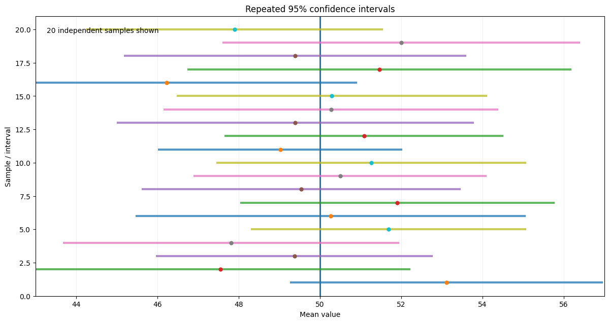
Featured visual: repeated samples generate different confidence intervals around a fixed population mean.

A confidence interval calculator estimates a range around a sample result that reflects uncertainty about an unknown population parameter. The calculation is usually easy; choosing the right method and interpreting the result correctly are the parts that matter most.

If a sample mean is 15 cm, for example, a 95% confidence interval might be 13.99 to 16.01 cm. The interval adds information that the single estimate cannot: how precise the estimate is under the statistical model and sampling assumptions.

Confidence Interval Calculator

The HTML version delivered with this document includes a working browser-based confidence interval calculator. It supports one-sample means and binomial proportions, uses Student's t when the population standard deviation is unknown, and offers Wilson as the default proportion method with Wald available for comparison.

Calculator inputs and method selection

What you are estimating	Inputs	Typical method
Population mean, σ known	Sample mean, population SD, sample size, confidence level	Z interval
Population mean, σ unknown	Sample mean, sample SD, sample size, confidence level	Student's t interval
Population proportion	Successes, total observations, confidence level	Wilson score by default; other binomial methods when required
Mean from raw observations	Individual measurements and confidence level	Calculate x̄ and s, then use the appropriate t procedure

Result design: show the point estimate, confidence limits, method name, critical value, standard error or equivalent uncertainty measure, margin of error when symmetric, and a brief “Why this method?” explanation.

What Is a Confidence Interval in Simple Terms?

A confidence interval is a range calculated from sample data by a statistical procedure designed to contain an unknown population parameter at a stated long-run rate, such as 95%.

The sample statistic at the center of the analysis is the point estimate. A confidence interval adds uncertainty around that estimate. If two studies both estimate a mean of 15, but one reports [14.9, 15.1] and another reports [11, 19], those studies are not equally informative. The first estimate is much more precise, assuming both analyses and study designs are valid.

What does a 95% confidence interval mean?

The 95% belongs to the procedure, not to a probability assigned to the fixed parameter after the data have been observed. If the same sampling process and 95% interval procedure were repeated many times, about 95% of those intervals would contain the true parameter under the model assumptions. NIST describes confidence levels in this repeated-sampling framework.

Micro-answer: A 95% confidence interval does not mean “there is a 95% chance the true mean is inside this particular interval.” A conventional frequentist statement is that we are 95% confident in the procedure that generated the interval.

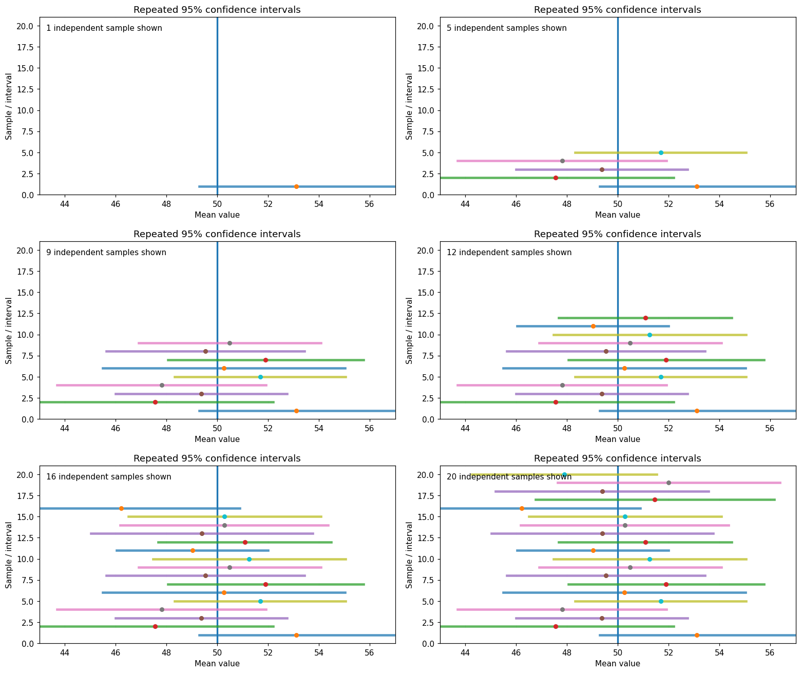
Animation: independent samples produce different intervals while the true population mean stays fixed. The animation is supplementary; the text above contains the full interpretation. Motion may not play in every Word viewer; compatible Word versions preserve the embedded GIF.

Why Confidence Intervals Matter

Confidence intervals make uncertainty visible. A point estimate alone can imply more exactness than the data justify, while an interval shows how much sampling variability remains.

That matters in research and decisions because the same estimated effect can support different conclusions depending on its precision. A mean difference of 5 units with a narrow interval around 5 is different from a mean difference of 5 with an interval that stretches from a meaningful negative effect to a large positive effect.

The practical question is therefore not only “Is the estimate above or below a null value?” It is also “Which values remain compatible with the data, and would those values lead to different decisions?”

How a Confidence Interval Works

Many familiar confidence intervals can be understood through the same structure:

Confidence interval = point estimate ± margin of error

Margin of error = critical value × standard error

The point estimate is the sample statistic, such as x̄ for a mean or p̂ for a proportion. The standard error describes how much that estimator is expected to vary from sample to sample. The critical value is determined by the selected confidence level and sampling distribution.

For a sample mean when the sample standard deviation is used, the familiar standard error is:

SE(x̄) = s / √n

Standard error and standard deviation are different. Standard deviation describes the spread of observations. Standard error describes uncertainty in an estimator such as the sample mean.

Confidence Interval Formulas for Means and Proportions

Mean when the population standard deviation is known

CI = x̄ ± z* (σ / √n)

This z interval uses the population standard deviation σ. NIST notes that population standard deviations are usually unknown in practice and need to be estimated from data.

Mean when the population standard deviation is unknown

CI = x̄ ± t* n−1 (s / √n)

When σ is unknown and replaced by the sample standard deviation s, the standard one-sample interval uses Student's t with n − 1 degrees of freedom. Penn State derives this t interval directly from the statistic (x̄ − μ)/(s/√n).

Proportion: Wald and Wilson are not the same method

The simplest textbook formula for a sample proportion is the Wald interval:

p̂ ± z* √[p̂(1 − p̂) / n]

Its simplicity is useful for learning, but it is not a universally reliable default. NIST says the normal approximation has poorer nominal coverage than alternative proportion methods and should be restricted to sufficiently large samples when p̂ is not near 0 or 1. Wilson is one of the alternatives NIST documents.

For 2 successes in 10 observations, the 95% Wald interval is approximately [−0.048, 0.448], which extends below the logically possible value of zero. The 95% Wilson interval is approximately [0.057, 0.510]. The difference is methodological, not a rounding error.

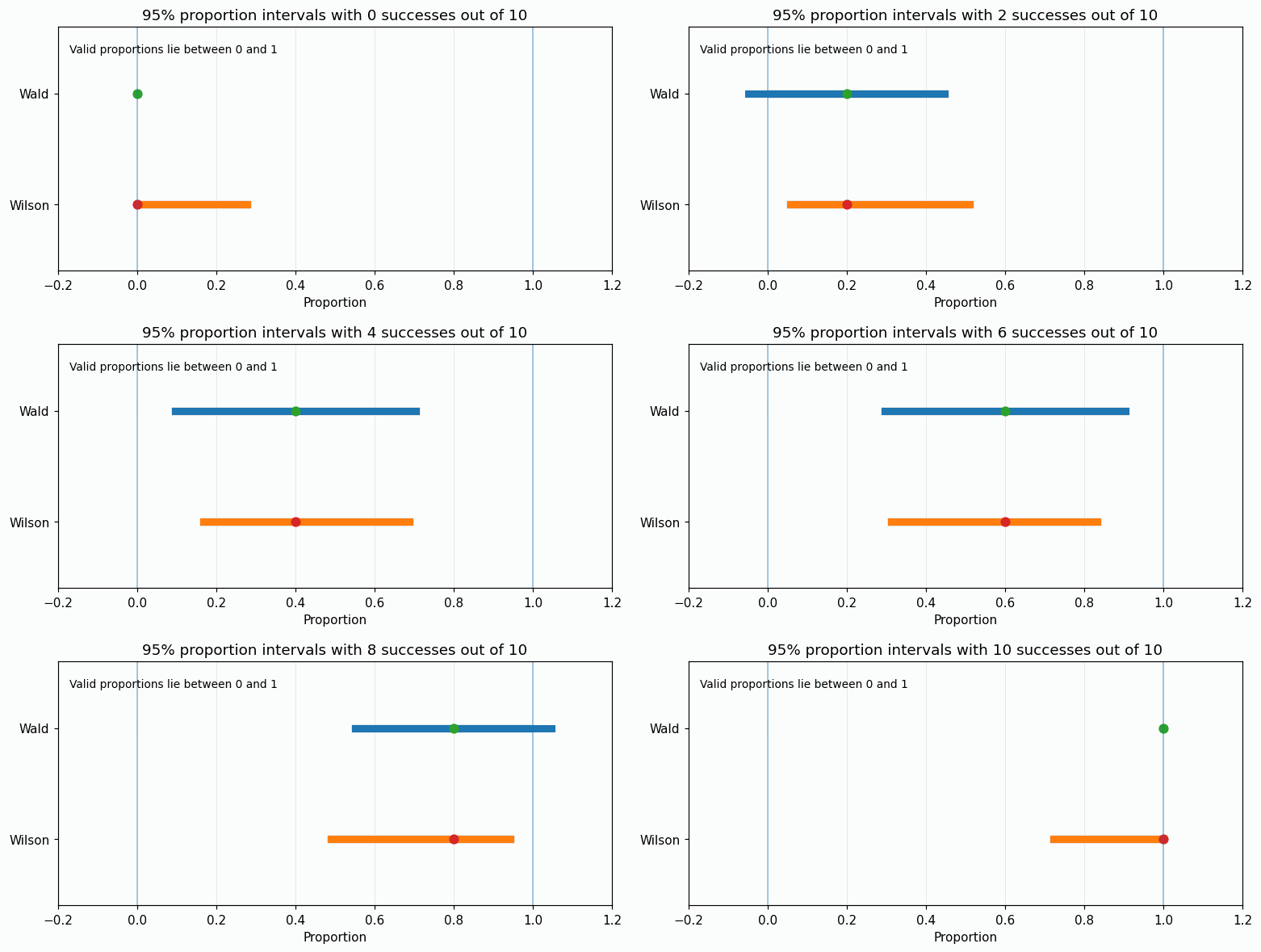
Animation: Wald and Wilson intervals can differ substantially near the 0 and 1 boundaries, especially with only ten observations. Motion may not play in every Word viewer; compatible Word versions preserve the embedded GIF.

Z-Interval vs. T-Interval: Which Should You Use?

The cleanest decision rule for a one-sample mean starts with one question: Is the population standard deviation σ genuinely known?

Situation	Recommended approach	Why
Population σ known	Z interval	The standard error uses the known population variability.
Population σ unknown and estimated with s	T interval	The t distribution accounts for uncertainty introduced by estimating σ.
Large n, σ unknown	T remains appropriate	The t critical value approaches z as degrees of freedom increase, so results become very similar.

The common rule “use z whenever n ≥ 30” is a classroom shortcut, not the fundamental statistical distinction. When σ is unknown, using t remains principled; for large samples, it simply makes little numerical difference. Penn State likewise describes t as the standard choice when σ is unknown.

For small samples, the assumptions deserve more attention. The exact classical t result assumes a normal population. With larger samples, the sampling distribution of the mean can be approximately normal under broad conditions, but severe skew, influential outliers, dependence, clustering, or complex sampling can make a simple one-sample t interval inadequate.

Confidence Levels and Critical Values

Confidence level	α	Two-sided z critical value
90%	0.10	1.645
95%	0.05	1.960
99%	0.01	2.576

A higher confidence level requires a larger critical value, so the interval becomes wider when the data and sample size stay fixed. A 99% interval is therefore not automatically “better” than a 95% interval. It gives greater long-run coverage but lower precision in the sense of a wider range.

For t intervals there is no single 95% critical value. The value depends on degrees of freedom, which is why software or a t table is used.

How to Calculate a Confidence Interval Step by Step

Suppose 49 randomly selected plants have a sample mean height of 15 cm and a sample standard deviation of 3.5 cm. We want a two-sided 95% confidence interval for the population mean.

The standard error is 3.5/√49 = 0.5. Because σ is unknown, use Student's t with 48 degrees of freedom. The 95% t critical value is approximately 2.0106, giving a margin of error of 2.0106 × 0.5 = 1.0053.

95% CI = 15 ± 1.0053 = [13.9947, 16.0053] cm

Rounded sensibly, report the result as mean = 15.00 cm, 95% CI [13.99, 16.01].

This calculation is only one part of validity. The interval assumes that the data and sampling design justify this t procedure. A perfectly executed formula does not repair a biased sample or dependent observations.

What Determines the Width of a Confidence Interval?

For many common intervals, three factors dominate width: sample size, variability, and confidence level.

Sample size

For a sample mean, SE = s/√n. As n increases, the standard error decreases. Because n is under a square root, halving the standard error requires roughly four times as many observations, assuming variability stays similar.

Variability

Larger s or σ produces a larger standard error and therefore a wider interval. Highly variable outcomes are harder to estimate precisely.

Confidence level

Moving from 90% to 95% to 99% increases the critical value and widens the interval. Lowering the confidence level narrows the interval, but it changes the long-run coverage rather than improving the data.

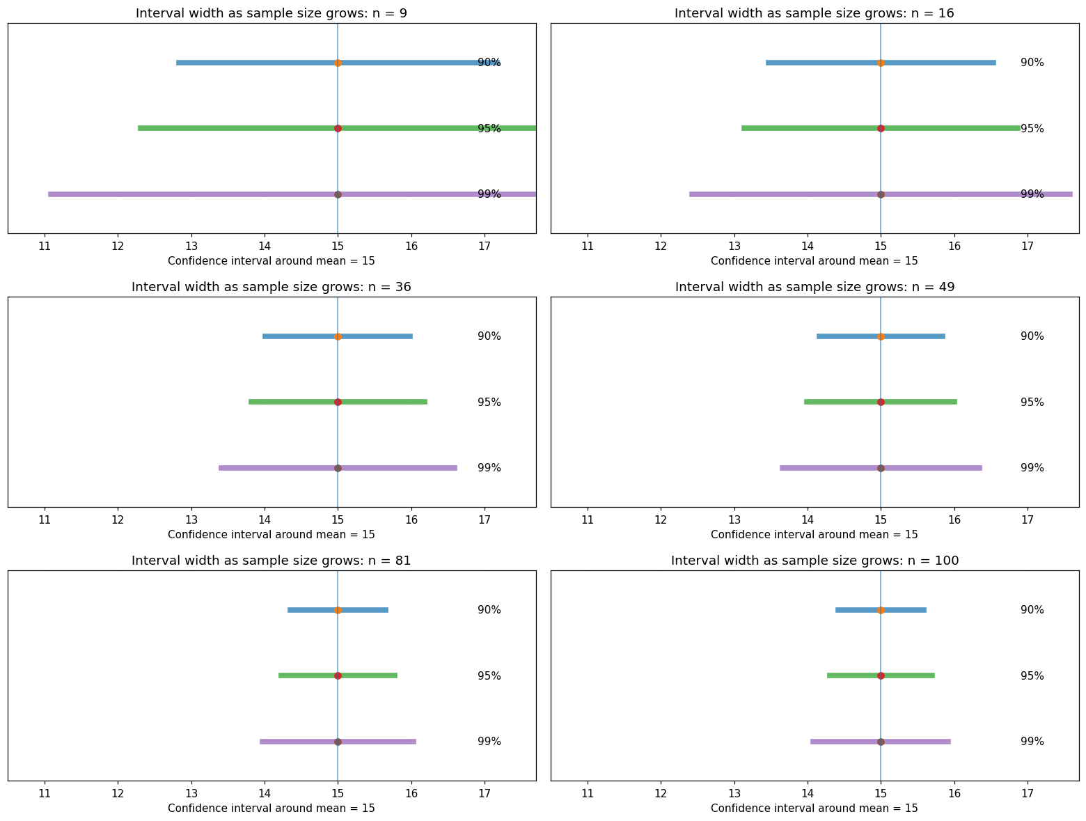
Animation: increasing sample size narrows each interval, while higher confidence levels remain wider for the same data. Motion may not play in every Word viewer; compatible Word versions preserve the embedded GIF.

Reality check: A very narrow confidence interval is not proof that the result is correct. More observations reduce sampling uncertainty, but they do not automatically fix selection bias, nonresponse, measurement error, confounding, or a systematically unrepresentative sample.

How to Interpret a Confidence Interval Correctly

When an interval includes zero

For a difference, such as a difference in means or regression coefficient, zero is often the null value. If a two-sided 95% interval includes zero, the corresponding two-sided test at α = 0.05 generally will not reject a zero effect when the test and interval are based on the same model and assumptions.

That does not prove there is no effect. A wide interval may include zero and also include effects large enough to matter.

When a ratio interval includes 1

For risk ratios, odds ratios, hazard ratios, and other ratio measures, the usual null value is 1. An interval crossing 1 is compatible with no relative difference at that confidence level, subject to the model used.

Narrow vs. wide intervals

A narrow interval generally means higher statistical precision. A wide interval means the estimate is less precise, often because the sample is small, variability is high, or a high confidence level was chosen.

Neither width alone tells you whether the estimate is unbiased. Statistical precision and study validity are separate issues.

Statistical significance vs. practical importance

An interval can exclude the null value while containing only effects too small to matter in practice. Conversely, an interval can include the null while also including large, decision-relevant effects. A useful interpretation considers the point estimate, interval width, null value, and a meaningful practical threshold rather than reducing the result to “significant” or “not significant.”

Confidence Interval vs. Related Statistical Measures

Concept	What it answers
Confidence interval	How uncertain is an estimated population parameter under the chosen procedure?
Margin of error	How far does a symmetric interval extend from the point estimate?
Standard error	How much is the estimator expected to vary across samples?
Standard deviation	How spread out are individual observations?
P-value	How compatible are the observed data with a specified null model, according to the chosen test?
Prediction interval	What range reflects uncertainty for a future individual observation or prediction?
Bayesian credible interval	What range contains a stated amount of posterior probability for a parameter under a specified model and prior?

A confidence interval for a mean should not be used as if it described where 95% of individual observations fall. That is a different problem, often addressed by a prediction interval or other distributional summary.

Common Confidence Interval Mistakes and Limitations

Using the 95% probability interpretation

The population parameter is fixed in the usual frequentist framework. The confidence level describes repeated performance of the procedure, not a probability attached to this one fixed interval after it has been observed.

Using z simply because the sample is “large”

If σ is unknown and s is used, t remains the natural one-sample mean procedure. The distinction matters most at small n, but the logic remains the same at large n.

Confusing a confidence interval with the data range

“Heights ranged from 9 to 22 cm” reports the observed minimum and maximum. A confidence interval around the mean answers a different question about uncertainty in a population parameter.

Ignoring study design

A conventional CI does not automatically account for biased sampling, nonresponse, measurement problems, clustering, repeated measures, survey weights, or confounding. In many real studies these issues have a larger impact than whether the critical value was rounded to three or four decimals.

Using the Wald proportion interval at the boundaries

For 0 successes in 10 trials, the Wald formula produces [0, 0], implying no uncertainty. A 95% Wilson interval is approximately [0, 0.278], which better reflects how little ten observations can establish. This is why proportion-method selection is not a cosmetic software setting.

Why Two Confidence Interval Calculators Can Give Different Answers

Different results do not automatically mean one calculator is broken. First compare the method names and assumptions.

Source of difference	What changes
Z vs. t	Critical value, especially with small samples
Wald vs. Wilson vs. Clopper-Pearson	Center, width, and boundary behavior for proportions
One-sided vs. two-sided intervals	How α is allocated and which bound is calculated
Continuity correction	Approximation used for discrete counts
Finite population correction	Standard error when sampling a substantial fraction of a finite population without replacement
Complex survey or clustered methods	Standard error accounting for the actual design
Rounding	Small differences in the displayed endpoints

The right troubleshooting question is therefore: “Which statistical procedure generated this interval?” not merely “Which calculator gives the number I expected?”

How Confidence Intervals Are Used in Real Research

In surveys, intervals around means or proportions quantify sampling uncertainty but do not repair nonresponse or a biased sampling frame. In clinical trials, confidence intervals commonly accompany treatment effects such as mean differences or ratio measures, and readers should consider both statistical and clinically meaningful thresholds.

In A/B testing, the useful interval is often for the difference between conversion rates rather than two unrelated intervals around each arm. In regression, intervals around coefficients communicate plausible magnitudes under the fitted model. In meta-analysis, forest plots display study estimates and intervals together so effect size and precision are visible at a glance.

For machine learning, the interval method must match the evaluation design. Treating cross-validation folds as independent observations can understate or otherwise misrepresent uncertainty because the folds are related through reused data and model fitting. The general lesson is that the formula must follow the data-generating and evaluation process.

Calculating Confidence Intervals in R, Python, Excel, and SPSS

R: t.test() returns confidence intervals for common t-test procedures. When reproducing a result, check whether you are doing a one-sample, paired, or two-sample analysis and which confidence level is specified.

Python: SciPy t-test result objects provide a confidence_interval() method for supported t-test results. Statsmodels exposes several binomial proportion interval methods, including normal/Wald, Agresti-Coull, Clopper-Pearson via beta, Wilson, and Jeffreys. This is a useful reminder that “a proportion confidence interval” is not one universal formula.

Excel: Microsoft documents CONFIDENCE.T for a Student's t based confidence amount and CONFIDENCE.NORM for a normal-distribution calculation. These functions return an amount to add to and subtract from a sample mean rather than a fully formatted pair of bounds.

SPSS: t-test and model procedures can report confidence intervals for their corresponding estimates. When results differ from another tool, check the exact procedure, options, corrections, and assumptions rather than comparing endpoints alone.

Frequently Asked Questions About Confidence Intervals

What is a confidence interval in one sentence?

It is a range calculated from sample data using a statistical procedure designed to capture an unknown population parameter at a stated long-run frequency.

Is a 90% or 95% confidence interval better?

Neither is universally better. A 90% interval is narrower but has lower long-run coverage; a 95% interval is wider and has higher coverage. The appropriate level depends on the decision and reporting context.

Can a confidence interval contain negative values?

Yes, when the parameter can logically be negative, such as a difference or regression coefficient. A negative lower bound is a warning sign when the parameter itself cannot be negative and the chosen approximation permits impossible values.

Can a proportion confidence interval go below 0 or above 1?

The simple Wald approximation can. That is one reason Wilson or other binomial procedures are often preferable, especially near the boundaries.

What happens when sample size increases?

All else equal, standard error decreases at approximately the rate 1/√n, so the confidence interval narrows. Quadrupling n roughly halves the standard error for a mean.

How large should a sample be?

There is no universal minimum. Required sample size depends on the parameter, variability, desired precision, confidence level, distribution, and sampling design. Planning a study for a target margin of error is a separate task from calculating an interval after data have been collected.

What if two 95% confidence intervals overlap?

Overlap by itself is not a reliable test of whether two parameters differ. Calculate an interval or formal test for the difference using a method that reflects the relationship between the samples.

Can a confidence interval be too wide to be useful?

Yes. If the interval contains values that would lead to very different actions, the estimate may be too imprecise for the decision even if a binary significance test gives a convenient label.

Is a confidence interval the same as a credible interval?

No. A frequentist confidence interval describes the long-run behavior of an interval procedure. A Bayesian credible interval represents posterior uncertainty about a parameter under a specified probability model and prior.

Quick Summary: How to Use a Confidence Interval Calculator Well

A confidence interval calculator should help you choose the correct statistical procedure, not merely turn four numbers into two endpoints. For a one-sample mean, use a z interval when σ is genuinely known and a t interval when σ is estimated using the sample standard deviation. For a binomial proportion, recognize that Wilson, Wald, and exact methods are different procedures with different behavior.

The most important practical insight is that calculation correctness, statistical validity, and study validity are three separate questions. A formula can be calculated perfectly while the sampling design is poor, and a narrow interval can be precisely wrong when systematic bias dominates sampling error.

After calculating the interval, check the method, assumptions, width, null value, and any threshold that would change the real decision. If the interval is too wide, the next sensible step is often a sample-size or margin-of-error calculation for future data collection rather than lowering the confidence level simply to make the interval look more precise.