
CPI Analysis Python Tutorial
Build one repeatable BLS workflow for headline inflation, core CPI, short term momentum, charts, validation, and monthly updates.
CPI Analysis Python Tutorial
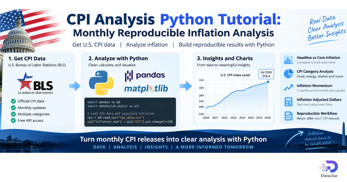
Methods note: Monthly rates use seasonally adjusted CPI. Standard 12-month rates use not seasonally adjusted CPI. Current example data are from the July 2026 BLS release.
A good CPI analysis should be easy to rerun, easy to audit, and clear about which inflation measure it uses. This CPI Analysis Python Tutorial builds that workflow with official U.S. Bureau of Labor Statistics data, Python, pandas, and matplotlib. The goal is not just to draw a chart once. The goal is to create a monthly process that can be repeated after every CPI release.
The current example uses the July 2026 CPI release, published August 12, 2026, with source review on September 8, 2026. In July, headline CPI rose 0.1 percent from the prior month on a seasonally adjusted basis and 3.4 percent over 12 months before seasonal adjustment. Core CPI rose 0.2 percent for the month and 2.5 percent over 12 months. Those numbers answer different questions, so the tutorial keeps their seasonal treatment and time windows separate.
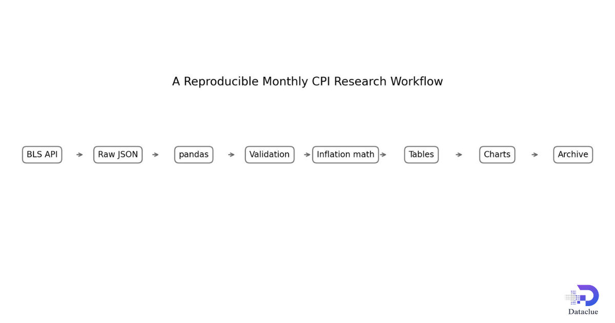
You will fetch series with the BLS Public Data API, save the raw response, convert observations into a clean monthly table, calculate several inflation rates, compare headline and core measures, inspect major categories, adjust dollar values for inflation, and archive each monthly run. The code is designed to be understandable first, then reusable.
In this guide
- Understand CPI Before You Calculate Inflation
- Set Up a Reproducible Python Inflation Project
- Choose BLS Series and Retrieve Monthly CPI Data
- Clean, Validate, and Reshape the Monthly Time Series
- Calculate Monthly, Annual, and Short-Term Inflation Momentum
- Compare Headline, Core, and Major CPI Categories
- Adjust Dollar Values for Inflation and Build Publication-Ready Plots
- Update, Audit, Reproduce, and Report the Analysis Each Month
Understand CPI Before You Calculate Inflation
The Consumer Price Index tracks average price change for a market basket of goods and services purchased by consumers. The CPI-U covers urban consumers and is the main population measure used in this tutorial. BLS also publishes CPI-W for urban wage earners and clerical workers, plus a chained CPI that uses a different formula for changing spending patterns.
An index level is not an inflation rate. An index such as 333.918 tells you where the price index stands relative to its base period. Inflation comes from the percentage change between index levels. That difference matters because a steadily high index can exist even when the current inflation rate is slowing.
Headline and core CPI answer different questions
Headline CPI includes the full consumer basket. Core CPI commonly means all items less food and energy. Core is often used to look past some short-term food and energy swings, but it does not mean food and energy are unimportant. A useful monthly review normally shows both.
Seasonal adjustment changes how you should calculate rates
For a standard change from the prior month, use a seasonally adjusted index. Seasonal adjustment removes recurring calendar patterns so short-term movement is easier to read. For the familiar 12-month CPI rate in the BLS release, use the not seasonally adjusted index. Mixing those conventions without explanation makes a dashboard harder to compare with official reporting.
Table 1. CPI measures and the question each one answers
| Measure | Basic calculation | Best use |
|---|---|---|
| CPI index level | Published index value | Track the price level over time |
| Monthly inflation | Current SA index compared with prior month SA index | Read short-term monthly movement |
| 12-month inflation | Current NSA index compared with the same month one year earlier | Match the standard BLS annual comparison |
| 3-month annualized | Compound the SA index change over three months to a 12-month rate | Measure recent momentum |
| 6-month annualized | Compound the SA index change over six months to a 12-month rate | Measure medium term momentum |
| Annual average change | Compare one calendar year average with another | Study average price levels across years |
CPI is broad, but it is not a perfect description of every household. Spending patterns differ by family, location, age, housing situation, and many other factors. CPI also describes price change. It does not by itself prove why prices changed.
Set Up a Reproducible Python Inflation Project
A reproducible project separates raw data, processed data, figures, tables, code, and metadata. That structure may feel like extra work at first, but it becomes valuable when a new release changes an old seasonally adjusted value or when you need to explain exactly how a chart was made.
Install the core tools
python -m pip install requests pandas matplotlib jupyterRequests handles the API call. pandas manages the monthly table and calculations. matplotlib makes the charts. pathlib keeps file paths readable. Jupyter gives you a convenient place to combine code, notes, checks, and output.
Keep the BLS key outside the notebook
import os
from pathlib import Path
from datetime import date

import requests
import pandas as pd
import matplotlib.pyplot as plt

BLS_API_KEY = os.getenv("BLS_API_KEY")
if not BLS_API_KEY:
    raise RuntimeError("Set BLS_API_KEY before the registered API request.")
BLS Version 2 requires registration. Registered Version 2 access currently allows up to 500 daily queries, 50 series in one query, and 20 years in one query. It also supports extra features such as calculations, annual averages, and catalog information. If you only need a small request, Version 1 can be used without registration, but its limits are lower.
Use a simple folder plan
project/
    notebooks/
    raw/
    processed/
    figures/
    tables/
    metadata/
Save the raw BLS response before any cleaning. A raw snapshot lets you compare releases later and makes it possible to trace a changed historical value back to the source data you originally received.
Choose BLS Series and Retrieve Monthly CPI Data
The most important choice in a CPI API request is the series ID. The ID identifies the population, item, area, periodicity, and seasonal status. Do not copy an old code into a new tutorial without checking it. Series metadata can change, and the seasonal status of some components is reviewed each year.
Table 2. Series dictionary for the main tutorial
| Readable name | Seasonal status | BLS series ID | Main role |
|---|---|---|---|
| Headline CPI-U all items | Seasonally adjusted | CUSR0000SA0 | Monthly change and momentum |
| Headline CPI-U all items | Not seasonally adjusted | CUUR0000SA0 | 12-month change and dollar adjustment |
| Core CPI | Seasonally adjusted | CUSR0000SA0L1E | Monthly core change and momentum |
| Core CPI | Not seasonally adjusted | CUUR0000SA0L1E | Core 12-month change |
| Food | Seasonally adjusted | CUSR0000SAF1 | Category monthly change |
| Energy | Seasonally adjusted | CUSR0000SA0E | Category monthly change |
| Shelter | Seasonally adjusted | CUSR0000SAH1 | Category monthly change |
| Medical care | Seasonally adjusted | CUSR0000SAM | Category monthly change |
| Transportation | Seasonally adjusted | CUSR0000SAT | Category monthly change |
| Apparel | Seasonally adjusted | CUSR0000SAA | Category monthly change |
Start with four series, not a huge list
import os
import requests
from datetime import date

URL = "https://api.bls.gov/publicAPI/v2/timeseries/data/"

series_ids = [
    "CUSR0000SA0",
    "CUSR0000SA0L1E",
    "CUUR0000SA0",
    "CUUR0000SA0L1E",
]

end_year = date.today().year
start_year = max(end_year - 5, 2000)

payload = {
    "seriesid": series_ids,
    "startyear": str(start_year),
    "endyear": str(end_year),
    "registrationkey": os.getenv("BLS_API_KEY"),
}

response = requests.post(URL, json=payload, timeout=30)
response.raise_for_status()
result = response.json()

if result.get("status") != "REQUEST_SUCCEEDED":
    raise RuntimeError(result.get("message", "BLS request failed"))

series = result.get("Results", {}).get("series", [])
if not series:
    raise RuntimeError("BLS returned no series data")
The API response stores each requested series as a list of observations. BLS often returns recent observations first, so do not assume the response is already in chronological order. Also inspect the message field. An invalid series can return an empty series with a message that explains the problem.
Turn each response into a tidy table
def tidy_bls_series(result, retrieval_date):
    rows = []
    for series in result["Results"]["series"]:
        sid = series["seriesID"]
        for obs in series.get("data", []):
            footnotes = "; ".join(
                f.get("text", "")
                for f in obs.get("footnotes", [])
                if f.get("text")
            )
            rows.append({
                "series_id": sid,
                "year": obs["year"],
                "period": obs["period"],
                "period_name": obs.get("periodName"),
                "value": obs["value"],
                "footnotes": footnotes,
                "retrieval_date": retrieval_date,
            })
    return pd.DataFrame(rows)
The optional cpi Python package can simplify common inflation adjustment tasks. PyPI lists version 2.0.10 as the current release from January 2026. Use it as a convenience, not as a reason to hide the CPI ratio or skip source checks.
Clean, Validate, and Reshape the Monthly Time Series
Economic time series code should fail clearly when the data are incomplete. A clean chart is not enough. You also need to know whether every month exists, whether values are numeric, and whether the source returned an unusual footnote.
Convert BLS period codes into real dates
def clean_monthly_cpi(df):
    out = df[df["period"].str.fullmatch(r"M(0[1-9]|1[0-2])")].copy()
    out["month"] = out["period"].str[1:].astype(int)
    out["date"] = pd.to_datetime({
        "year": out["year"].astype(int),
        "month": out["month"],
        "day": 1,
    })
    out["value"] = pd.to_numeric(out["value"], errors="coerce")
    out["series_id"] = out["series_id"].astype("string")
    out = out.sort_values(["series_id", "date"]).reset_index(drop=True)
    return out
The filter keeps only M01 through M12. BLS can also return annual average records such as M13 when those are requested or available. Treat annual averages as a separate product rather than pretending they are another month.
Check duplicates, missing dates, and missing values
def quality_report(df):
    duplicate_count = int(df.duplicated(["series_id", "date"]).sum())
    missing_calendar_months = 0

    for _, group in df.groupby("series_id"):
        dates = pd.DatetimeIndex(group["date"].dropna().unique()).sort_values()
        if dates.empty:
            continue
        expected = pd.date_range(dates.min(), dates.max(), freq="MS")
        missing_calendar_months += len(expected.difference(dates))

    return pd.DataFrame([{
        "rows": len(df),
        "first_month": df["date"].min(),
        "last_month": df["date"].max(),
        "missing_calendar_months": missing_calendar_months,
        "missing_numeric_values": int(df["value"].isna().sum()),
        "duplicate_series_months": duplicate_count,
    }])

def complete_monthly_calendar(df):
    if df.duplicated(["series_id", "date"]).any():
        raise ValueError("Resolve duplicate series-month rows before reindexing")

    frames = []
    for series_id, group in df.groupby("series_id", sort=False):
        group = group.set_index("date").sort_index()
        expected = pd.date_range(group.index.min(), group.index.max(), freq="MS")
        group = group.reindex(expected)
        group.index.name = "date"
        group["series_id"] = series_id
        frames.append(group.reset_index())

    return pd.concat(frames, ignore_index=True)
The quality report now distinguishes two problems: an observation can be present with a nonnumeric or unavailable value, or a calendar month can be absent as a row. Run the report first, resolve duplicates, and then use complete_monthly_calendar() before calculating rates. Reindexing to a monthly calendar makes an absent month explicit as a missing value, so a one-, three-, six-, or twelve-row shift still corresponds to the intended number of calendar months.
Do not automatically replace a missing official CPI observation with a guess. The October 2025 all items and core indexes are a useful real example. BLS did not publish those main estimates because CPI data collection was disrupted during the 2025 lapse in appropriations. The API represents unavailable October observations with a missing marker and an explanatory footnote.
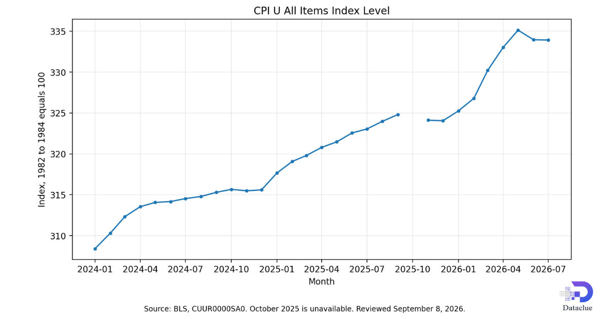
The visible gap in the index chart is useful information. Hiding it with interpolation would make the time series look smoother, but it would remove part of the data history that a reproducible analysis should preserve.
Calculate Monthly, Annual, and Short-Term Inflation Momentum
Once the index table is clean, calculate each rate from the index level that matches the question. Keep full precision during the calculation. Round only when you prepare the display table.
Use separate formulas for separate questions
Use seasonally adjusted CPI for the standard monthly change. The formula compares this month with the immediately preceding month.
Use the not seasonally adjusted series when you want to match the standard 12-month BLS headline convention.
The annualized rates compound the full 3-month or 6-month index change to a 12-month pace. Do not take one monthly rate and simply multiply it by 12. Short-term annualized inflation is a momentum measure, not a forecast of the next year. The helper above first converts a date-indexed series to an explicit monthly frequency, preserving gaps as missing values rather than silently shifting across them.
def as_monthly_series(s):
    if not isinstance(s.index, pd.DatetimeIndex):
        raise TypeError("CPI series must use a DatetimeIndex")
    return s.sort_index().asfreq("MS")

def monthly_change(s):
    s = as_monthly_series(s)
    return 100 * s.pct_change(1, fill_method=None)

def twelve_month_change(s):
    s = as_monthly_series(s)
    return 100 * s.pct_change(12, fill_method=None)

def annualized_momentum(s, months):
    if months not in (3, 6):
        raise ValueError("Use 3 or 6 months for this momentum measure")
    s = as_monthly_series(s)
    periods_per_year = 12 / months
    return 100 * ((s / s.shift(months)) ** periods_per_year - 1)
Table 3. Latest inflation dashboard for July 2026
| Measure | Headline | Core | Series treatment |
|---|---|---|---|
| Monthly change | 0.1% | 0.2% | Seasonally adjusted |
| 12-month change | 3.4% | 2.5% | Not seasonally adjusted |
| 3-month annualized | 0.49% | 1.64% | Seasonally adjusted index levels |
| 6-month annualized | 3.85% | 2.42% | Seasonally adjusted index levels |
The July 2026 snapshot shows why one number cannot summarize inflation. Headline inflation was 3.4 percent over 12 months, but its 3-month annualized pace was about 0.49 percent. Core 12-month inflation was 2.5 percent, while its 3-month annualized pace was about 1.64 percent. The short window suggests recent momentum was softer than the 12-month headline rate, but that can change quickly.
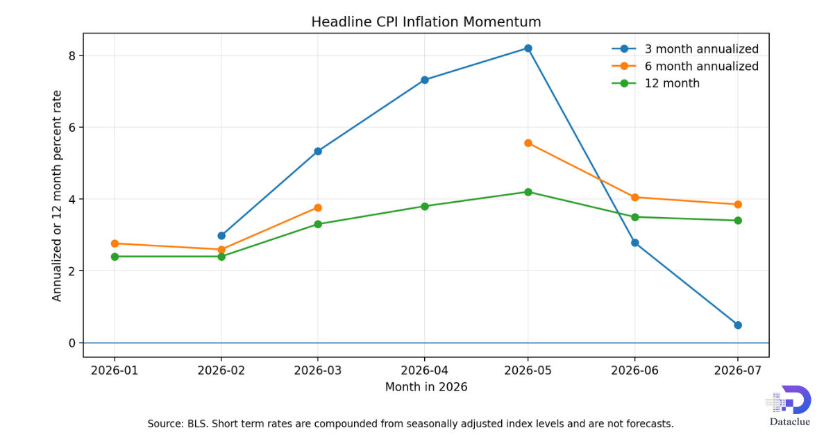 Figure 3. Short term annualized CPI momentum can change much faster than the 12-month rate.
Annual average inflation is different again. It compares the average CPI level for one calendar year with the average for another year. Do not call an annual average change a 12-month change, and do not call a December to December change an annual average.
Compare Headline, Core, and Major CPI Categories
Headline and core CPI are useful starting points, but category data help explain where price movement is concentrated. Keep the comparison descriptive. A category growth rate is not the same thing as that category contribution to the total CPI change, because contribution also depends on its relative importance in the consumer basket.
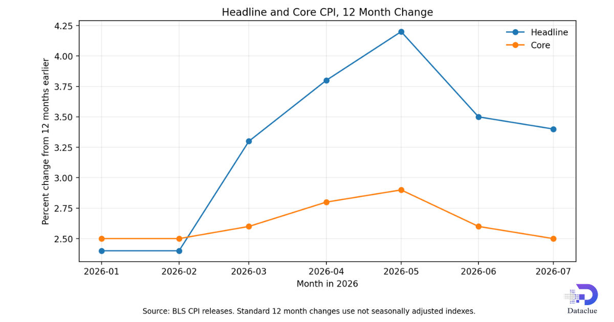
During the first seven months of 2026, headline 12-month inflation moved above core inflation as energy prices increased sharply. By July, the headline rate was 3.4 percent and the core rate was 2.5 percent. That difference is consistent with the energy index rising 14.7 percent over the same 12-month period.
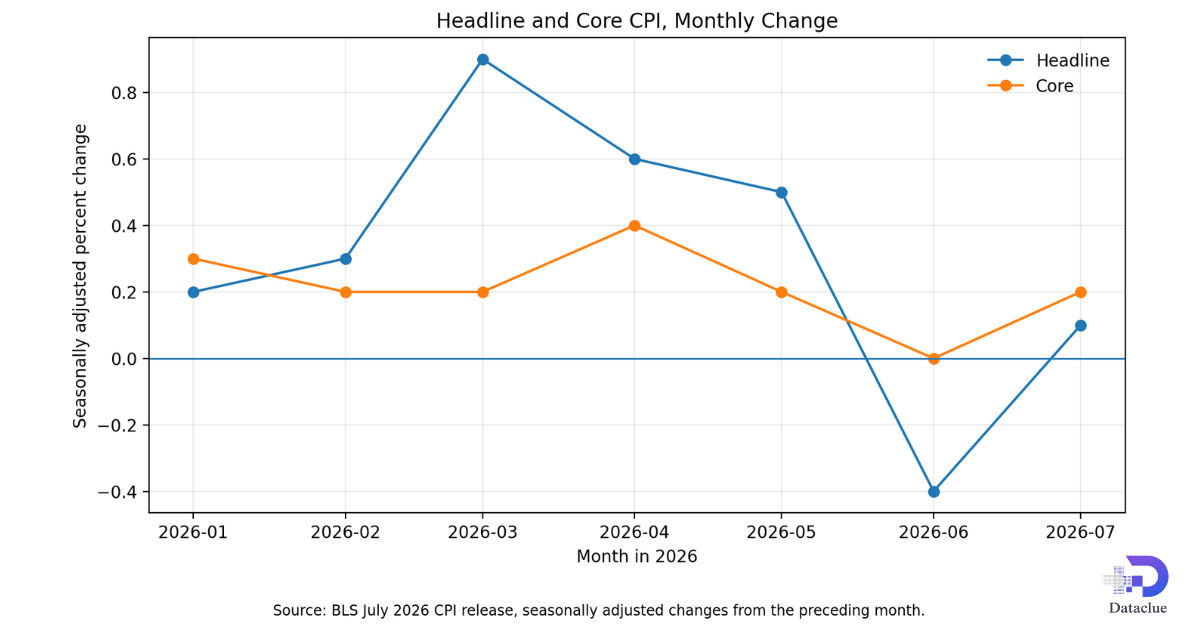
The monthly chart tells a different story. Headline CPI fell 0.4 percent in June and rose only 0.1 percent in July, while core CPI was unchanged in June and rose 0.2 percent in July. Short term monthly values can be noisy, so use them with the longer trend rather than in isolation.
Table 4. Major CPI category snapshot for July 2026
| Category | Monthly change | 12-month change | SA series | NSA series |
|---|---|---|---|---|
| All items | 0.1% | 3.4% | CUSR0000SA0 | CUUR0000SA0 |
| Core | 0.2% | 2.5% | CUSR0000SA0L1E | CUUR0000SA0L1E |
| Food | 0.1% | 3.0% | CUSR0000SAF1 | CUUR0000SAF1 |
| Energy | -1.5% | 14.7% | CUSR0000SA0E | CUUR0000SA0E |
| Shelter | 0.1% | 3.2% | CUSR0000SAH1 | CUUR0000SAH1 |
| Medical care | 0.4% | 1.7% | CUSR0000SAM | CUUR0000SAM |
| Transportation | -0.5% | 5.8% | CUSR0000SAT | CUUR0000SAT |
| Apparel | 0.1% | 3.9% | CUSR0000SAA | CUUR0000SAA |
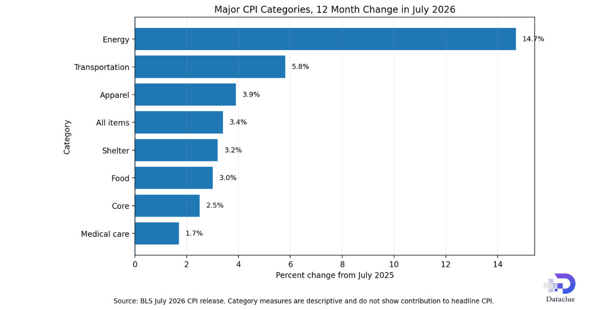
Figure 6. Latest 12-month category inflation. A category rate is not the same as its contribution to headline CPI.
Energy stands out in the July 12-month comparison. Transportation also ran above headline inflation, while medical care was below it. These differences are useful for describing the pattern, but a simple correlation between categories would not tell you which one caused headline inflation. It also would not measure each category contribution.
Define event windows before you inspect the result
If you want to study a pandemic period, an energy shock, a policy change, or another event, choose the dates before you look at the chart. Then describe what changed during that window. A time series chart can show timing and association. It does not by itself identify a causal mechanism.
Adjust Dollar Values for Inflation and Build Publication-Ready Plots
Inflation adjustment converts a nominal amount from one price level into an equivalent amount at another price level. Use the same compatible CPI series at the source and target dates.
For a simple monthly example, the not seasonally adjusted all items CPI was 325.252 in January 2026 and 333.918 in July 2026. A January amount of $100 therefore equals about $102.66 in July 2026 dollars when this broad CPI measure is used.
def adjust_for_inflation(amount, source_cpi, target_cpi):
    if source_cpi <= 0 or target_cpi <= 0:
        raise ValueError("CPI values must be positive")
    return amount * target_cpi / source_cpi

value = adjust_for_inflation(100, 325.252, 333.918)
print(round(value, 2))
Over a longer window, $100 in January 2024 corresponds to about $108.27 in July 2026 dollars using the same not seasonally adjusted all items series. The calculation is transparent, which makes it easy to audit.
Use the cpi package as an optional shortcut
# Optional monthly example. Refresh the package data before using current CPI.
from datetime import date
import cpi

cpi.update()
monthly_adjusted = cpi.inflate(
    100,
    date(2024, 1, 1),
    to=date(2026, 7, 1),
)
The package documentation states that its bundled BLS data do not update automatically, so run cpi.update() before relying on it for current observations. It also supports month-to-month adjustments when dates are supplied as datetime.date objects. As of the September 8, 2026 source review, PyPI lists version 2.0.10, released January 13, 2026. For monthly publication work, the direct BLS workflow still gives you clearer control over the observation date, seasonal status, raw response, and revision history.
Make every plot answer one question
A publication-ready CPI chart should name the measure, time window, unit, source, series treatment, and retrieval date. Use a zero reference line when rates can be positive or negative. Keep the time axis chronological. Do not cut the chart at a convenient date simply because older data weaken a narrative.
Update, Audit, Reproduce, and Report the Analysis Each Month
The biggest advantage of a reproducible CPI workflow appears one month later. Instead of rebuilding the analysis, change the end date, fetch the new response, run the same validation, compare the new snapshot with the prior snapshot, and regenerate the tables and figures.
Use reusable fetch and calculation functions
from pathlib import Path
import json
from datetime import datetime, timezone

def fetch_bls(series_ids, start_year, end_year, api_key):
    payload = {
        "seriesid": series_ids,
        "startyear": str(start_year),
        "endyear": str(end_year),
        "registrationkey": api_key,
    }
    response = requests.post(
        "https://api.bls.gov/publicAPI/v2/timeseries/data/",
        json=payload,
        timeout=30,
    )
    response.raise_for_status()
    result = response.json()
    if result.get("status") != "REQUEST_SUCCEEDED":
        raise RuntimeError(result.get("message"))
    return result, payload

def save_raw_snapshot(result, raw_dir):
    stamp = datetime.now(timezone.utc).strftime("%Y%m%dT%H%M%SZ")
    path = Path(raw_dir) / f"bls_cpi_{stamp}.json"
    path.parent.mkdir(parents=True, exist_ok=True)
    path.write_text(json.dumps(result, indent=2), encoding="utf-8")
    return path
Audit revisions instead of overwriting history silently
BLS recalculates seasonal factors each year and may revise the previous five years of seasonally adjusted CPI history. In February 2026, revised seasonally adjusted indexes were published for 2021 through 2025. That means an old monthly chart can differ from a new download even when your code has not changed.
def revision_audit(old_df, new_df):
    keys = ["series_id", "date"]
    merged = old_df.merge(
        new_df, on=keys, how="inner", suffixes=("_old", "_new")
    )
    merged["revision"] = merged["value_new"] - merged["value_old"]
    return merged[merged["revision"].abs() > 0].copy()
Save both the old and new snapshots. If a historical value changes, report the revision in a small audit file. This is much better than replacing history without a note.
Table 5. Reproducibility log for the article snapshot
| Field | Recorded value |
|---|---|
| Source review date | September 8, 2026 |
| Latest observation used | July 2026 |
| Release date | August 12, 2026 |
| API pattern | BLS Public Data API Version 2 POST request |
| Main monthly series | CUSR0000SA0 and CUSR0000SA0L1E |
| Main 12-month series | CUUR0000SA0 and CUUR0000SA0L1E |
| Raw file practice | Save timestamped JSON before cleaning |
| Processed file practice | Save tidy CSV or Parquet separately |
| Revision practice | Compare historical SA values with the prior snapshot |
| Known missing period | October 2025 for main all items and core CPI |
Common problems and practical fixes
Table 6. Troubleshooting guide
| Problem | What to check |
|---|---|
| BLS request fails | HTTP status, API status field, message field, key, year span, and query limits |
| Series is empty | Series ID spelling, seasonal status, item definition, and supported dates |
| Latest month is missing | Release calendar, source messages, and whether the observation is published yet |
| Monthly rate looks wrong | Confirm that the calculation uses the seasonally adjusted series |
| 12-month rate differs from BLS headline | Confirm that the comparison uses the not seasonally adjusted series |
| Momentum rate is extreme | Check the full index span and compound formula before interpreting it |
| Old values changed | Run the seasonal revision audit and preserve both snapshots |
Frequently asked questions
How do I get CPI data into Python?
bls_data_api.fredapilibrary with your personal API key. [1, How do I calculate inflation or changes over time?
.pct_change() method.What CPI series should I use for monthly U.S. inflation?
For the standard all items monthly change, use the seasonally adjusted CPI-U all items series, CUSR0000SA0.
What series should I use for the standard 12-month headline rate?
Use the not seasonally adjusted CPI-U all items series, CUUR0000SA0, when you want to match the familiar BLS 12-month convention.
Is a 3-month annualized rate a forecast?
No. It describes the pace implied by the most recent three month index change if that pace were compounded for a year. Future inflation can be very different.
Why can an old seasonally adjusted CPI value change?
BLS recalculates seasonal factors each year and can revise the previous five years of seasonally adjusted indexes.
Should I fill a missing CPI month with interpolation?
Not in an official published analysis unless you have a clearly stated research reason. Preserve the source gap and document it.
Can I use CPI to adjust money from one date to another?
Yes. Multiply the original amount by the target CPI divided by the source CPI, using a compatible series and clearly stated dates.
Does a category correlation show what caused headline inflation?
No. Correlation describes co-movement. It does not measure contribution and it does not establish cause.
Monthly rerun checklist
- Confirm the new CPI observation has been released.
- Update the request end year only when needed.
- Fetch the same verified series IDs.
- Save the raw JSON with a timestamp before cleaning.
- Run duplicate, missing month, numeric, and latest month checks.
- Recalculate monthly, 12-month, 3-month, and 6-month measures.
- Compare historical seasonally adjusted values with the prior snapshot.
- Regenerate the dashboard, category table, and charts.
- Save processed data, figures, package versions, and metadata.
- Write the observation month and retrieval date in every published output.
Final takeaway
A useful CPI analysis is more than a chart of the latest number. It is a small research system. Keep the source official, use the right seasonal treatment, calculate each time window from the correct index, preserve missing data, audit revisions, and save enough metadata to reproduce the result next month. That approach makes the analysis easier to trust and easier to maintain.
Methods and sources
This tutorial uses official U.S. Bureau of Labor Statistics CPI definitions and the Public Data API request pattern. The current data example uses the July 2026 CPI release. Monthly changes use seasonally adjusted series. Standard 12-month changes use not seasonally adjusted series. Short term momentum is compounded from seasonally adjusted index levels. The source review date is September 8, 2026.
- U.S. Bureau of Labor Statistics, Consumer Price Index, July 2026 release
- U.S. Bureau of Labor Statistics, Public Data API FAQs
- U.S. Bureau of Labor Statistics, Seasonal Adjustment in the CPI
- U.S. Bureau of Labor Statistics, 2025 federal government shutdown impact on CPI
- PyPI, cpi package, version 2.0.10, released January 13, 2026
- cpi documentation, monthly adjustments and updating the local BLS dataset
- Google Search Central, Creating Helpful, Reliable, People First Content
Downloads
Files attached to this article for your reference.