
Factor Analysis: Types, Steps, Assumptions & Uses
Factor analysis is a statistical method for explaining relationships among observed variables through a smaller number of underlying, unobserved dimensions called factors. It is useful when many measurements appear to…
Factor Analysis: Types, Steps, Assumptions & Uses
Factor analysis is a statistical method for explaining relationships among observed variables through a smaller number of underlying, unobserved dimensions called factors. It is useful when many measurements appear to reflect broader constructs such as satisfaction, mathematical ability, anxiety, service quality, or perceived value.
The method is powerful, but the practical challenge is not pressing the “Factor Analysis” button in software. The important work is deciding whether the data are suitable, choosing an extraction method, deciding how many factors to retain, selecting a defensible rotation, and interpreting the solution without relying on arbitrary cutoffs.
What Is Factor Analysis in Simple Terms?
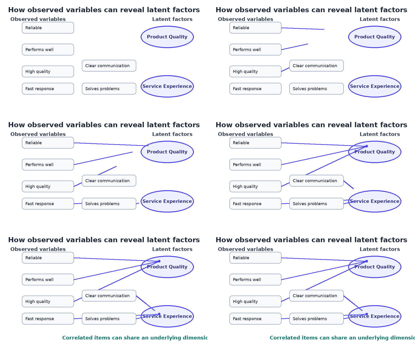
In simple terms, factor analysis asks whether a large set of correlated measurements can be explained by a smaller set of common dimensions. A factor is called latent because it is not observed directly; instead, researchers infer it from the pattern of relationships among measured variables. Source
Imagine a customer survey with questions about product reliability, product performance, staff responsiveness, problem resolution, price fairness, and value for money. The individual answers are observed variables. If related questions move together, the analysis may reveal broader factors such as Product Quality, Service Experience, and Perceived Value.
That distinction matters because a factor is not simply another column already present in the dataset. It is a statistical construct used to account for shared variation among the observed indicators.
Why Factor Analysis Is Used
Researchers use factor analysis when the observed variables contain meaningful overlap and the goal is to understand the structure behind that overlap. In questionnaire development, exploratory factor analysis can help reveal which items appear to belong together before a stricter measurement model is tested. Source
The method can also simplify a large measurement system. Instead of discussing 30 closely related survey items individually, an analyst may be able to describe a smaller number of interpretable dimensions. In psychology and education those dimensions may represent traits or abilities; in market research they may represent quality perceptions, service experience, trust, or price sensitivity.
This reduction should not be confused with automatic improvement. A weak questionnaire does not become valid merely because software extracts factors. Poor item wording, inadequate sampling, missing constructs, weak correlations, and unstable factors remain measurement problems that require judgment.
Core Factor Analysis Terms You Need to Understand
A few terms appear repeatedly in every factor analysis output. Understanding them before looking at software tables prevents some of the most common interpretation errors.
| Term | Simple meaning | Why it matters |
|---|---|---|
| Factor | An unobserved underlying dimension | Represents the construct inferred from several measurements |
| Observed variable | A directly measured item or variable | Provides the evidence used to infer factors |
| Factor loading | The relationship between an observed variable and a factor | Shows how strongly an item is associated with a factor |
| Communality | The proportion of an item’s variance represented by the common factors | Shows how well the common-factor solution represents that item |
| Uniqueness | Variance not represented by the common factors | Captures item-specific and error-related variation |
| Eigenvalue | A quantity associated with variance captured by a dimension | Often appears in decisions about how many dimensions to retain |
| Scree plot | A graph of eigenvalues by factor number | Helps visualize where additional factors contribute less |
| Factor score | An estimated score for an observation on a factor | Can sometimes be carried into later analysis |
| Rotation | A transformation of the factor axes | Can make the loading pattern easier to interpret |
Factor Loadings, Communalities, and Factor Scores Are Not the Same Thing
A factor loading describes the relationship between an observed variable and a factor. A communality summarizes how much of an item’s variance is represented by the common factors taken together. A factor score, by contrast, estimates where a particular respondent or observation lies on a factor. Source
These quantities answer different questions. Confusing a factor loading with a factor score can lead to incorrect reporting, especially when factor scores are later used in regression, clustering, or other analyses.
Exploratory vs Confirmatory Factor Analysis
Exploratory Factor Analysis, or EFA, is appropriate when the underlying structure is uncertain and the analyst wants to investigate how items group together. Confirmatory Factor Analysis, or CFA, begins with a specified measurement structure and evaluates how well that structure is supported by the data. Source
In practice, the difference is not simply “early research versus advanced research.” It is a difference in the question being asked. EFA asks what plausible structure is present; CFA asks whether a specified structure is consistent with the observed covariance pattern under a defined model.
| Feature | EFA | CFA |
|---|---|---|
| Main purpose | Discover plausible structure | Test a specified measurement structure |
| Prior structure | Limited or uncertain | Defined in advance |
| Item-factor relationships | Explored | Constrained by the model |
| Common use | Scale development and structure discovery | Scale validation and measurement testing |
| Typical framework | Exploratory factor model | Structural equation modeling measurement model |
Factor Analysis vs PCA: What Is the Difference?
Factor analysis and Principal Component Analysis are often presented together because both can reduce a large set of variables to fewer dimensions. Statistically, however, they do not have the same objective.
PCA constructs components from the observed variables in order to summarize observed variance efficiently. Common factor analysis models the shared relationships among variables through latent factors and distinguishes common variance from variance that remains unique to an indicator. UCLA’s factor-analysis guidance explicitly separates PCA’s use of total observed variance from common-factor methods that model shared variance. Source
A practical decision rule is more useful than arguing over labels. Choose PCA when the main objective is compression or representation of the observed variables. Choose common factor analysis when the scientific question concerns latent constructs that are intended to explain shared relationships among measurements.
PCA is also not a form of confirmatory factor analysis. CFA specifies a latent measurement model in advance, while PCA constructs components from the observed variables. Treating those procedures as interchangeable blurs a major methodological distinction. Source
| Factor analysis | PCA |
|---|---|
| Models latent factors behind shared relationships | Constructs components from observed variables |
| Focuses on common structure | Summarizes observed variance |
| Includes a conceptual distinction between common and unique variance | Does not model measurement error in the same way |
| Useful for construct-oriented questions | Useful for data compression and representation |
What Are the Assumptions of Factor Analysis?
There is no single assumption checklist that applies identically to every extraction and estimation method. The basic requirement is that the variables contain meaningful shared relationships. If almost every variable is unrelated to every other variable, there is little common structure for a factor model to explain.
Relationships represented with conventional correlation-based methods should also be reasonably compatible with the type of correlation being analyzed. Perfect multicollinearity and singularity are problematic because duplicate or exact linear combinations of variables do not provide independent measurement information.
Independent observations are normally assumed in standard applications unless the model explicitly handles clustered or repeated data. Outliers, severe response artifacts, miscoding, and missing-data patterns can distort the correlations that drive the solution.
Multivariate normality requires more nuance. It is especially relevant for conventional maximum-likelihood inference, but factor analysis is not limited to a single estimator. The lavaan package, for example, documents maximum-likelihood, generalized least squares, weighted least squares, diagonally weighted least squares, unweighted least squares, and robust variants for different modeling conditions. Source
How Large Should the Sample Be?
Fixed rules such as “five respondents per item” or “ten respondents per item” are easy to remember but too crude to guarantee a stable factor solution. Classic simulation work by MacCallum and colleagues showed that sample requirements depend on features such as communalities and how strongly each factor is determined by its indicators. Source
The practical implication is that sample size should be judged together with measurement quality. A simple, strongly determined structure with high communalities can behave very differently from a weak structure containing poorly represented items. A ratio alone cannot capture that difference.
How Do You Know Whether Your Data Is Suitable for Factor Analysis?
Begin with the correlation structure. The variables should show enough shared association to make a common-factor explanation plausible, but they should not simply be duplicates of one another.
Kaiser-Meyer-Olkin Test Explained
The Kaiser-Meyer-Olkin measure evaluates sampling adequacy by comparing the magnitude of observed correlations with the magnitude of partial correlations. Values closer to 1 generally indicate a more favorable pattern for common-factor modeling. Source
A value around .60 is often treated as a rough lower screening guideline in applied work, but it should not be used as an automatic pass/fail law. A marginal result should prompt closer inspection of individual items, the correlation pattern, sample quality, and the substantive reason for keeping each variable.
Bartlett's Test of Sphericity Explained
Bartlett's test evaluates whether the correlation matrix differs from an identity matrix. If the matrix were effectively an identity matrix, the variables would offer very little shared correlation structure for factor extraction. A significant result supports factorability, but it does not prove that the resulting factors will be meaningful, stable, or theoretically coherent. Source
How to Perform Factor Analysis Step by Step
A defensible workflow starts with the research question rather than with software defaults. First define the construct or measurement problem and select variables that have a substantive reason to be analyzed together. Then screen the data for coding errors, missingness, distributions, unusual response patterns, and the measurement level of the items.
Next, inspect the correlation matrix and evaluate factorability with diagnostics such as KMO and Bartlett’s test where appropriate. Choose an extraction method that matches the research objective and the characteristics of the data. Determine the number of factors using multiple sources of evidence rather than a single rule.
After extraction, choose a rotation that reflects whether the factors may reasonably correlate. Examine the loading pattern, communalities, cross-loadings, weak items, and factor correlations. Review problematic items using statistical evidence and substantive meaning together. Finally, name the factors, estimate factor scores only if they are actually needed, validate the structure where possible, and report each major decision transparently.
This sequence matters because the stages are connected. An inappropriate factor count changes the rotation; the rotation changes the apparent loading pattern; item removal changes the correlation matrix; and every one of those choices can alter the final interpretation.
Which Factor Extraction Method Should You Use?
Principal Axis Factoring is a common starting point when the goal is to investigate shared latent structure rather than summarize total observed variance. Maximum Likelihood factor analysis is useful when likelihood-based estimation and related inferential procedures are appropriate for the data and model assumptions. Source
Other methods include minimum-residual, least-squares, alpha, and image-factoring approaches. IBM SPSS and R packages such as EFAtools expose multiple extraction methods, which is useful but also creates a responsibility: the analyst should know why a method is being chosen instead of accepting whichever option appears first in a menu. Source
| Research goal or condition | Practical starting point | Main consideration |
|---|---|---|
| Investigate shared latent structure | Principal Axis Factoring | Focuses on common variance |
| Likelihood-based modeling with suitable data | Maximum Likelihood | Relies on stronger distributional/model assumptions for standard inference |
| Ordinal questionnaire items | Ordinal-aware correlation or estimation workflow | Measurement scale and estimator matter |
| Pure data compression | Principal Component Analysis | Not the same latent-variable objective as common factor analysis |
How Many Factors Should You Retain?
Choosing the number of factors is one of the most consequential decisions in exploratory factor analysis. Retaining too few factors can merge distinct constructs; retaining too many can create unstable or uninterpretable dimensions.
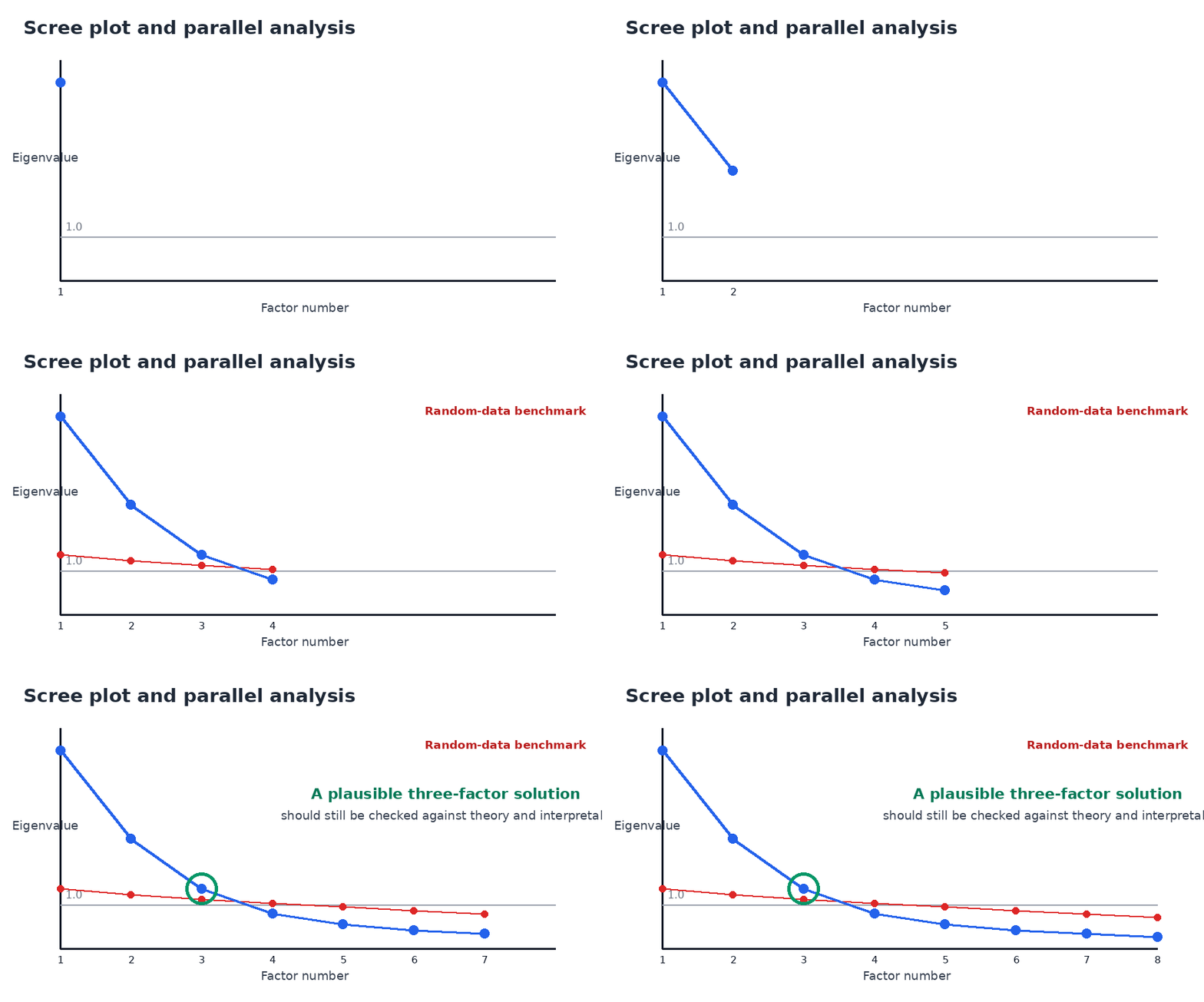
The Kaiser criterion retains factors or components with eigenvalues greater than 1. It is easy to calculate, but it should not be treated as a standalone truth. A scree plot adds visual information by showing where the eigenvalue curve begins to flatten, although the location of the “elbow” can be ambiguous.
Parallel analysis provides another source of evidence by comparing observed eigenvalues with those expected from random data. Methodological research has repeatedly supported parallel analysis as a useful alternative to relying solely on the eigenvalue-greater-than-one rule. Source
The strongest decision framework combines retention evidence with theory and interpretability. If the Kaiser rule suggests four factors, the scree plot suggests three, and parallel analysis suggests two, do not force one rule to “win.” Compare the solutions, ask whether each retained factor is well determined, and check whether the factor structure makes substantive sense.
Factor Rotation Explained: Varimax, Oblimin, and Promax
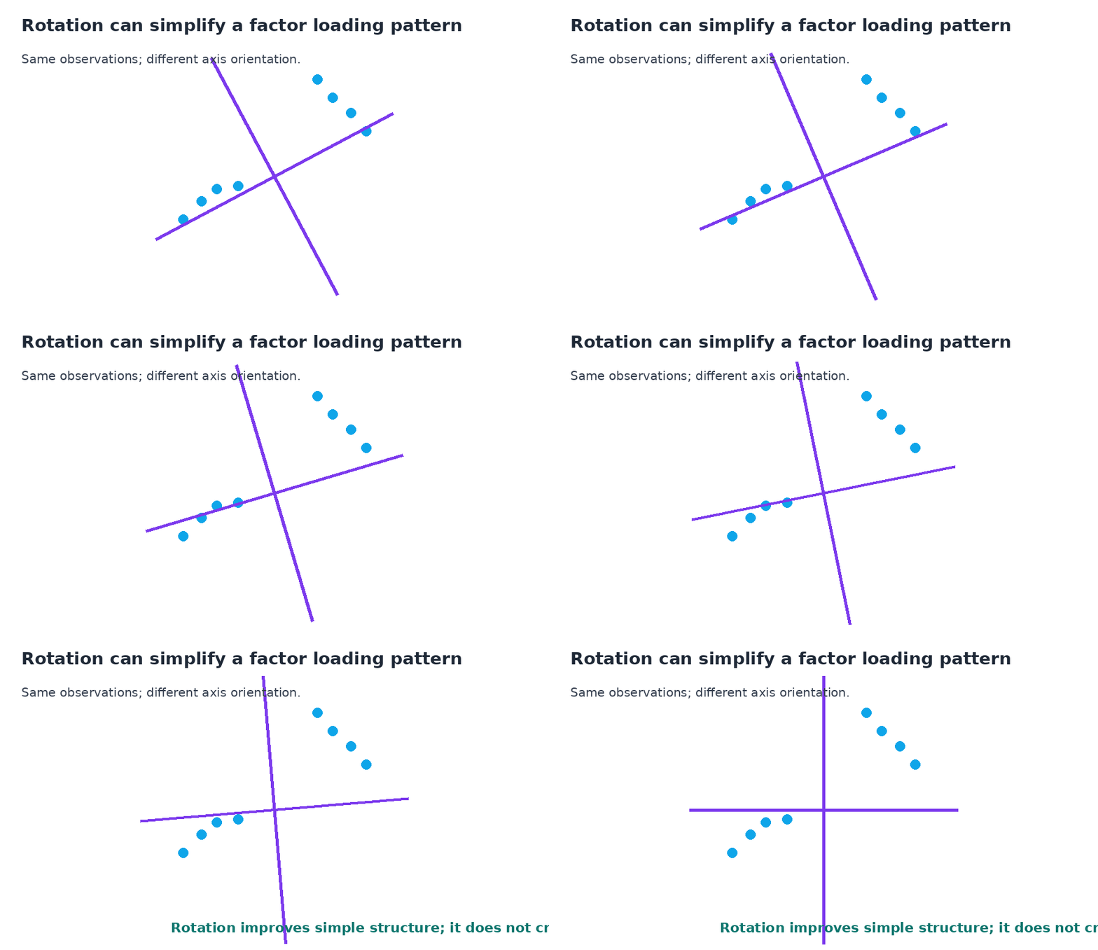
Rotation changes the orientation of the factor axes so that the loading pattern is easier to interpret. It does not create new observations or add information that was absent from the data. Source
Varimax is an orthogonal rotation, which means the rotated factors are constrained to remain uncorrelated. Direct Oblimin and Promax are oblique rotations, which allow factors to correlate. IBM SPSS documents both orthogonal and oblique rotation options. Source
Automatically choosing Varimax because it is familiar can be unrealistic. Constructs such as satisfaction and loyalty, engagement and motivation, or anxiety and depression may plausibly correlate. When theory and the observed solution support those relationships, an oblique rotation can be more defensible.
Oblique rotation also changes what must be interpreted. A pattern matrix contains regression-like relationships between indicators and factors, while a structure matrix contains indicator-factor correlations. Those matrices are identical when factors are orthogonal but can differ when factors correlate. Source
How to Interpret Factor Analysis Results
Interpretation should focus on the full pattern rather than one isolated cutoff. Larger absolute factor loadings generally indicate stronger relationships, but no single value automatically separates “good” from “bad” items in every discipline and sample.
Negative loadings indicate an inverse relationship with the orientation of the factor. They are not automatically evidence of a faulty item. Because the sign of a factor can often be reversed without changing the substantive model, the important issue is whether the direction is conceptually coherent across the items.
Cross-loadings deserve more attention than simple deletion rules usually allow. An item that loads on two factors may be ambiguously worded, may genuinely represent more than one construct, or may reveal that the two factors are not as distinct as expected. Removing the item can improve statistical simplicity while simultaneously weakening content validity.
Communalities show how well the retained common factors represent each item. Persistently low communalities can indicate that an item is poorly captured by the proposed factor structure and can contribute to unstable factor recovery in less favorable sampling conditions. Source
Factor naming is another judgment step. Software identifies a mathematical pattern, not the correct psychological, educational, or commercial label. A defensible name should reflect the content shared by the strongest indicators and the theory behind the measurement.
Factor Analysis Example: From Survey Questions to Latent Factors
Consider a hypothetical customer-experience questionnaire with items about product performance, service, and value. After suitable data screening and an exploratory factor analysis, imagine that the rotated loading pattern below is obtained. These values are illustrative and are not results from a real study.
| Survey item | Product Quality | Service Experience | Perceived Value |
|---|---|---|---|
| Product is reliable | .82 | .08 | .12 |
| Product performs well | .79 | .11 | .13 |
| Quality meets expectations | .76 | .14 | .18 |
| Staff respond quickly | .10 | .84 | .09 |
| Staff solve problems | .15 | .80 | .12 |
| Communication is clear | .16 | .73 | .17 |
| Price is reasonable | .11 | .09 | .81 |
| Product is worth the cost | .17 | .14 | .78 |
| Benefits justify the price | .19 | .16 | .74 |
How to Read the Example
The first three items load strongly on the first factor, the service items load on the second, and the value items load on the third. The weak secondary loadings make the hypothetical solution easy to interpret, so the labels Product Quality, Service Experience, and Perceived Value are reasonable.
Real datasets are often much less tidy. An item may load .48 on one factor and .42 on another; a theoretically important item may have a weak communality; or parallel analysis and the scree plot may point to different factor counts. Those situations cannot be resolved responsibly by a single threshold. They require a decision that combines statistical evidence with measurement theory and the purpose of the instrument.
How to Run Factor Analysis in SPSS, R, and Python
IBM SPSS Statistics provides a Factor procedure with several extraction methods, rotations, diagnostics, and factor-score options. It is approachable for users who prefer menus, but its convenience can encourage default-driven analysis. The method, factor count, and rotation still need to be justified. Source
R offers a particularly broad psychometric ecosystem. The psych package includes exploratory factor analysis and parallel-analysis functions, while lavaan is widely used for CFA and structural equation modeling. EFAtools provides additional workflows for screening, retention, extraction, and correlation choices. Source
Python users can work with scikit-learn’s FactorAnalysis class when a maximum-likelihood latent-variable model fits the task. The factor_analyzer package provides a more traditional EFA-oriented interface with extraction, rotation, KMO, Bartlett testing, and related utilities. Source
For beginners, SPSS may reduce the learning curve for basic output, while R often provides greater flexibility for psychometric workflows and reproducible research. Python is attractive when factor modeling must be integrated into a broader data-science pipeline. The best choice is the environment that supports the estimator, correlation type, diagnostics, rotation, and validation strategy the study actually needs.
Can Factor Analysis Be Used With Likert-Scale Data?
Yes, but treating every Likert-scale response as ordinary continuous data without considering its ordinal nature can be too simplistic. The appropriate workflow depends on the number of response categories, distributions, sample conditions, and the intended estimator.
For ordinal indicators, analysts may use polychoric correlations in exploratory work or categorical-data estimators in confirmatory models. The lavaan documentation, for example, allows binary and ordinal endogenous variables to be declared as ordered and describes a WLSMV-style workflow based on diagonally weighted least squares for estimation. Source
This does not mean that polychoric correlations or ordinal estimators are automatically superior in every dataset. They introduce their own assumptions and computational considerations. The broader lesson is that measurement level should influence the method rather than being ignored.
When Should You Use Factor Analysis?
Factor analysis is appropriate when the research question concerns underlying dimensions that may account for relationships among several observed measurements. Typical examples include psychological traits, educational abilities, patient-reported outcomes, organizational climate, customer perceptions, and questionnaire scale development.
It is less appropriate when the variables are largely unrelated, when the only goal is predictive accuracy, when variables have no substantive reason to reflect common constructs, or when the sample and measurement design cannot support a stable solution.
Another practical boundary is interpretability. If repeated analyses produce factors that are mathematically available but conceptually incoherent, adding more extraction and rotation options may not solve the underlying measurement problem. The variables themselves may need to be redesigned.
Common Factor Analysis Mistakes and Misconceptions
One common mistake is treating PCA and common factor analysis as interchangeable. Both reduce dimensions, but only the latter is explicitly framed around latent common factors and common variance. Source
A second mistake is retaining factors only because their eigenvalues exceed 1. Parallel analysis, scree evidence, theoretical coherence, factor strength, and interpretability provide a stronger basis for deciding dimensionality. Source
A third mistake is using Varimax automatically. Orthogonal rotation imposes uncorrelated factors, which may contradict the theory or the empirical relationships among constructs. Source
Rigid loading cutoffs create a similar problem. A loading threshold can be a useful descriptive convention, but it should not replace an assessment of communalities, cross-loadings, factor definition, item content, and the consequences of deletion.
Finally, EFA does not prove that a latent construct causes the observed items. The model provides a statistical representation of covariance; causal claims require a stronger research design and additional assumptions.
Advantages and Limitations of Factor Analysis
The major advantage of factor analysis is interpretive economy. A large set of overlapping measurements can sometimes be represented by a smaller number of coherent dimensions, making scale development and complex survey results easier to understand.
Its major limitation is that the solution is not self-interpreting. Variable selection, factor count, extraction, rotation, item deletion, correlation type, and sampling conditions can all affect the result. Different defensible choices can produce different but mathematically valid solutions.
There is also a trade-off between simple structure and construct coverage. Removing every cross-loading or weak item can make a table look cleaner while narrowing the construct until important content is lost. Statistical neatness and measurement validity are not always the same objective.
Theoretical best practice may also exceed what a real project can support. Independent validation samples, large ordinal models, sensitivity analyses, and multiple candidate solutions require more observations, time, software expertise, and reporting space. When resources are limited, the study should state those constraints instead of presenting an exploratory solution as more certain than it is.
How to Report Factor Analysis Results in Research
A useful report should make the major decisions reproducible. Describe the sample and variables, data screening, the correlation approach, KMO and Bartlett results where used, the extraction method, the evidence used to decide factor count, the rotation, the main loading pattern, communalities, problematic or removed items, and factor correlations when an oblique solution is used.
If factor scores are used later, state how they were estimated. If CFA or another validation step follows, report that analysis separately rather than implying that the exploratory procedure itself confirmed the structure.
A concise methods description might say: “An exploratory factor analysis was conducted using principal axis factoring. Factor retention was evaluated using parallel analysis, scree evidence, and theoretical interpretability. Because the proposed constructs were expected to correlate, an oblique rotation was used. Items were evaluated using their loading patterns, communalities, cross-loadings, and substantive relevance rather than a single automatic deletion threshold.”
FAQs
What is factor analysis in simple words?
It is a statistical method for identifying whether many observed variables can be represented by a smaller number of underlying factors. The factors are inferred from the relationships among measured variables rather than observed directly. Source
What is a good KMO value?
Higher KMO values are generally more favorable because they indicate that partial correlations are relatively small compared with the observed correlations. Around .60 is often used as a rough applied screening point, but it should not be treated as a universal pass/fail rule.
What does Bartlett's test tell you?
It evaluates whether the correlation matrix differs sufficiently from an identity matrix. A significant result supports the presence of shared correlation structure, although it does not guarantee that the final factor solution will be strong or interpretable. Source
What is a good factor loading?
There is no universal loading threshold for every study. Larger absolute loadings indicate stronger relationships, but interpretation should also consider sample quality, communalities, cross-loadings, factor definition, theory, and what would be lost by deleting the item.
How many factors should I retain?
Use several sources of evidence. Parallel analysis, the scree plot, theoretical coherence, factor strength, and interpretability usually provide a more defensible decision than relying on the eigenvalue-greater-than-one rule alone. Source
Should I use Varimax or Oblimin?
Use an orthogonal rotation such as Varimax when uncorrelated factors are a defensible assumption. Use an oblique method such as Oblimin or Promax when the underlying constructs may reasonably correlate. Source
Can factor analysis be used with Likert-scale data?
Yes, but ordinal response scales may justify ordinal-aware methods such as polychoric correlations or categorical-data estimators rather than automatically treating every item as continuous. Source
Can factor scores be used in regression?
They can be used in later analyses, including regression, but factor scores are estimates rather than perfectly observed variables. The scoring method and the consequences of estimation error should be considered and reported. Source
Factor Analysis: Key Takeaways and Next Steps
The best next step is to match the method to the research question before opening statistical software. Use exploratory factor analysis when the structure genuinely needs exploration, confirmatory factor analysis when a specified measurement structure is ready to be tested, and PCA when the primary objective is component-based data reduction rather than latent-construct modeling. Source
Then evaluate factorability, choose an extraction method that fits the data and objective, decide factor count using more than one source of evidence, select rotation according to whether the factors may correlate, and interpret loadings, communalities, cross-loadings, and factor meaning together.
The most useful conclusion is also slightly contrarian: good factor analysis is not produced by mechanically applying KMO greater than .60, eigenvalue greater than 1, a single loading cutoff, and Varimax. Those conventions can be useful starting points, but a defensible solution comes from combining statistical evidence, data-appropriate estimation, measurement theory, interpretability, and validation.
You May Also Like Multiple Regression
Try it in DataClue
Ready to run Factor Analysis?
Identify underlying latent variables that explain patterns in observed variables.
Run Factor Analysis