
Introduction to Statistics: A Complete Beginner Guide
Learn statistics step by step with a beginner guide covering data, variables, classification, frequency distributions, tables, formulas, and examples.
Introduction to Statistics: A Complete Beginner Guide With Examples, Tables, and Formulas
Statistics helps us turn a mass of facts into information we can understand. It gives us a clear way to collect data, arrange it, present it, analyze it, and interpret what it means. This guide follows the ideas taught in Chapter 1 of the supplied Business Mathematics and Statistics text. The language and examples are refreshed for beginners in the United States, but the scope stays with the chapter. By the end, you should be able to explain what statistics is, tell variables from attributes, compare primary and secondary data, classify observations, build frequency tables, and use the main formulas needed for grouped data.
Contents
- What Is Statistics?
- A Short History of Statistics
- The Statistical Method
- Definition of Statistics
- Characteristics of Statistics
- Limitations of Statistics
- Importance of Statistics in Different Fields
- Functions of Statistics
- Variables and Attributes
- Continuous and Discrete Variables
- Statistical Data
- Collection of Statistical Data
- Editing of Data
- Classification and Tabulation
- Types of Classification
- Important Class Terms
- Tabulation and Types of Tables
- Frequency Distribution
- How to Form a Frequency Distribution
- Relative Frequency and Relative Cumulative Frequency
- Bivariate Frequency Distribution
- Formula Guide
- Worked Example 1: Discrete Frequency Distribution
- Worked Example 2: Continuous Frequency Distribution
- Worked Example 3: Bivariate Frequency Distribution
- Chapter Summary
- Common Mistakes
What Is Statistics?
The word statistics is used in two main ways. In the plural sense, statistics means numerical facts. Examples include population counts, prices, sales, wages, exam results, and production figures. These are numbers that describe something.
In the singular or technical sense, statistics means a field of study. It is the set of methods used to collect, organize, present, analyze, and interpret numerical data. This second meaning is what students usually mean when they study statistics as a subject.
The chapter also makes an important point about large groups of facts. Statistics is most useful when we study an aggregate, which means a collection of observations, rather than one isolated case.
A Short History of Statistics
The chapter begins with a short history. It explains that statistical thinking grew from the need to record facts about states, populations, public activity, and social conditions. Over time, the subject became a scientific tool for many fields.
The chapter mentions Adolphe Quetelet for the development of social statistics, Francis Galton for work linked with heredity and measurement, Karl Pearson for major work in mathematical statistics, and William S. Gosset for early twentieth century statistical methods. The purpose of this history is simple. Statistics developed because people needed better ways to understand large sets of facts.
The Statistical Method
The statistical method is a sequence of steps. Each step prepares the data for the next one. If the first steps are weak, the final conclusion can also be weak.
- Collection of data. Gather the facts needed for the question.
- Classification and condensation. Arrange similar facts into useful groups.
- Presentation. Show the information in a clear form, such as text, a table, or a graph.
- Analysis. Study patterns, comparisons, and relationships in the data.
- Interpretation. Explain what the results mean in the context of the problem.
Definition of Statistics
A simple working definition is this: statistics is the science of collecting, organizing, presenting, analyzing, and interpreting numerical data for a useful purpose.
The definition is broader than doing calculations. A good statistical study begins before the numbers are analyzed. We must decide what information is needed, how it will be collected, and how it will be checked.
Characteristics of Statistics
The chapter describes several features that help us recognize statistical information. These features also explain why careful data work matters.
- Statistics deals with aggregates of facts rather than a single isolated observation.
- Statistical facts are expressed in numerical form.
- A reasonable standard of accuracy is needed when facts are counted or estimated.
- Statistical results are often affected by many causes at the same time.
- Statistical techniques work with information that can be reduced to quantitative form.
- Statistical methods are especially useful for handling a large mass of numerical data.
Limitations of Statistics
Statistics is powerful, but it has limits. The chapter warns students not to treat every numerical result as a perfect truth.
- Statistical laws are generally true on average. They may not describe every individual case.
- Statistics deals with aggregates. One person or one event may behave differently from the group.
- Statistics studies characteristics that can be stated numerically.
- Poor collection, analysis, or interpretation can produce misleading results.
- Statistical methods should not be applied carelessly to data that are not reasonably comparable or homogeneous.
- Expert knowledge is important because the same data can be misunderstood when methods are used incorrectly.
Importance of Statistics in Different Fields
The chapter gives statistics a wide role because many fields depend on facts, comparisons, and measured change. The exact method may differ from one field to another, but the need for reliable information is the same.
- Planning and public administration. Statistics helps governments estimate needs and study public problems.
- Agriculture. Crop output, rainfall, fertilizer use, and farm experiments can be studied with statistical methods.
- Industry. Managers can compare production, quality, costs, and demand.
- Business and commerce. Businesses use data to study sales, prices, customers, and market conditions.
- Insurance. Risk and past experience are studied through numerical records.
- Forecasting. Past information can help estimate future conditions, although a forecast is never certain.
- Social sciences. Statistics helps researchers study social conditions and relationships between measured variables.
- Physical and medical sciences. Experiments and measured outcomes often need statistical organization and comparison.
- Research. Statistics helps investigators summarize evidence and draw careful conclusions.
Functions of Statistics
The chapter also lists practical functions of statistics. These functions explain what statistics helps us do after data have been collected.
- Present facts in a clear and definite form.
- Simplify a large or complex set of information.
- Make comparisons easier.
- Help in the formation of policies and programs.
- Support forecasts about future conditions.
- Widen individual experience by bringing together many observations.
- Show the relative importance of facts.
- Help test scientific ideas and laws.
- Support work in other fields where numerical evidence is needed.
Variables and Attributes
A variable is a characteristic that can take different numerical values. Height, weight, age, weekly wages, and number of children are examples of variables.
An attribute is a quality that is described rather than measured directly as a numerical amount. Examples include beauty, honesty, color, or a category such as pass and fail. An attribute can still be counted by category, but the quality itself is not measured in the same way as height or weight.
| Feature | Variable | Attribute |
|---|---|---|
| Meaning | A characteristic that takes numerical values | A quality or category that is described |
| Examples | Height, weight, age, wages, number of children | Color, honesty, beauty, pass or fail category |
| Measured directly | Yes | Not in the same numerical sense |
Continuous and Discrete Variables
A continuous variable can, in theory, take any value between two points. Height and weight are common examples. A student can weigh 145 pounds, 145.2 pounds, or 145.25 pounds depending on the measuring tool.
A discrete variable takes separate countable values. The number of children in a family is discrete because values such as 2.4 children do not describe an actual count in one family. The number of students in a class is another example.
| Point of comparison | Continuous variable | Discrete variable |
|---|---|---|
| Possible values | Can take any value within a range | Takes separate countable values |
| Typical source | Measurement | Counting |
| Examples | Height, weight, time | Number of children, number of students |
Statistical Data
Data are recorded facts or measurements. Raw data are observations in the form in which they were first collected. Before we can study them easily, we often need to sort, classify, or tabulate them.
The chapter distinguishes discrete and continuous data in the same way it distinguishes discrete and continuous variables. Count data usually form discrete series. Measured data can be grouped into continuous classes.
Collection of Statistical Data
Data can come from primary or secondary sources. The difference depends on who collected the information and why it was collected.
Primary data are collected first hand for the current investigation. Secondary data were collected earlier by another person or organization and are later used for a new purpose. A data set can be primary for one study and secondary for another.
| Point | Primary data | Secondary data |
|---|---|---|
| Meaning | Collected first hand for the current study | Collected earlier for another purpose |
| Example | A class survey carried out today | A government table already published |
| Main caution | Collection must be planned and checked | Source, date, definition, and quality must be checked |
Editing of Data
Editing means checking the collected data before analysis. The goal is to find mistakes, omissions, unclear entries, and information that does not belong in the study.
Editing should happen before a researcher builds final tables. A small error in raw data can affect every later calculation.
Classification and Tabulation
Classification means arranging observations into groups or classes so that similar items are placed together. Classification makes a large data set easier to compare.
Tabulation means presenting data in rows and columns. A good table gives the information a clear order. It also prepares the data for analysis.
Types of Classification
Descriptive classification groups observations by attributes or qualities. Examples include residence type, employment status, or product category.
Numerical classification groups observations by measurable values such as height, weight, age, income, or exam marks.
A simple or one way classification uses one characteristic at a time. A two way classification uses two characteristics. A manifold classification uses more than two characteristics.
| Type | Basis | Simple example |
|---|---|---|
| Descriptive classification | Attribute or quality | Employment status |
| Numerical classification | Measurable numerical value | Age group |
| One way classification | One characteristic | Students by age group |
| Two way classification | Two characteristics | Students by height and weight group |
| Manifold classification | More than two characteristics | Students by age, program, and residence type |
Important Class Terms
Grouped data use several terms that students should know before they build a frequency distribution.
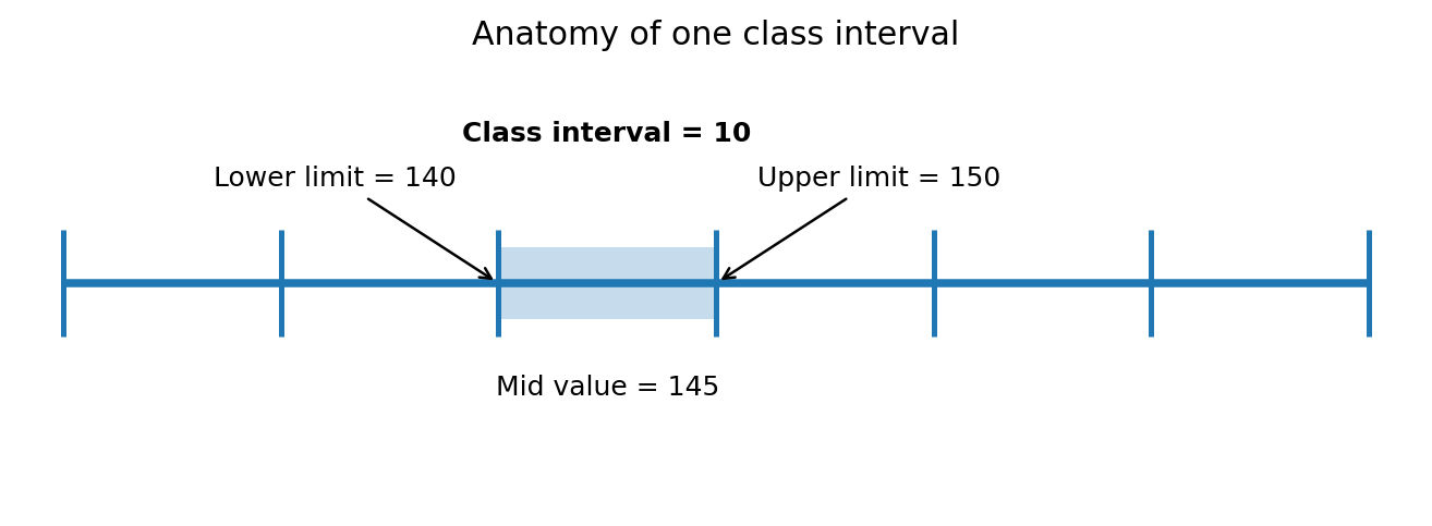
| Term | Meaning | Example using 140 to under 150 |
|---|---|---|
| Lower class limit | The starting value of a class | 140 |
| Upper class limit | The ending boundary of the class | 150 |
| Class interval | The size or width of the class | 10 |
| Mid value | The center of the class | 145 |
| Class frequency | The number of observations in the class | For example, 8 students |
Tabulation and Types of Tables
A statistical table is a systematic arrangement of numerical data in rows and columns. A simple table answers one main question. A two way table answers a question involving two variables. A higher order table can include more variables.
A good table should have a clear title, labeled rows and columns, and totals where they help the reader check the data.
| Table type | What it shows | Example |
|---|---|---|
| Simple table | One main characteristic | Students by program |
| Two way table | Two characteristics | Height group by weight group |
| Higher order table | More than two characteristics | Program by age group by residence |
Frequency Distribution
A frequency distribution shows how often values or groups of values occur. It changes a long list of observations into a more useful summary.
The chapter describes three forms. An individual series lists observations separately. A discrete series lists each countable value with its frequency. A continuous series groups measured values into class intervals.
| Series type | How observations appear | Example |
|---|---|---|
| Individual series | Each observation is listed separately | A short ordered list of marks |
| Discrete series | Each countable value has a frequency | Number of flowers on branches |
| Continuous series | Measurements are grouped into intervals | Student weights grouped into ten pound classes |
How to Form a Frequency Distribution
The chapter gives a practical sequence for building a grouped frequency distribution. First find the range. Next decide the number of classes. Then choose a suitable class interval. After that, write the classes, tally each observation, and count the tallies to obtain the frequency.
The number of classes should be large enough to show the shape of the data, but not so large that the table becomes difficult to read. The chapter uses Sturges formula as an approximate guide.
The sequence to follow
- Find the maximum and minimum values.
- Calculate the range.
- Estimate a useful number of classes.
- Choose a simple class interval.
- Write the class limits in order.
- Read each observation and place one tally in the correct class.
- Count the tallies and write the frequency.
- Check that the total frequency equals the total number of observations.
Relative Frequency and Relative Cumulative Frequency
Relative frequency shows the share of all observations that fall in one value or class. It is useful when two data sets have different totals because proportions are easier to compare than raw counts.
Cumulative frequency is a running total. Relative cumulative frequency turns that running total into a share of the full data set.
Bivariate Frequency Distribution
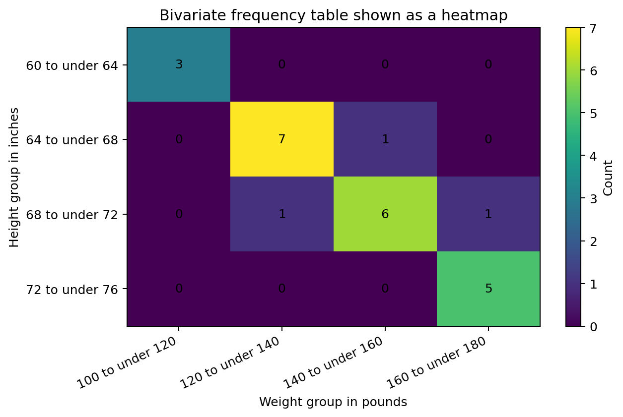
A bivariate frequency distribution classifies observations by two variables at the same time. The chapter uses examples such as height with weight and age of husband with age of wife.
In a bivariate table, the rows represent classes of one variable and the columns represent classes of the second variable. Each cell shows how many observations belong to that combination.
Formula Guide
Range tells us how far the data spread from the smallest value to the largest value.
This is the Sturges formula used in the chapter. Here m is the approximate number of classes and N is the number of observations. Use base 10 logarithm.
The result can be rounded to a simple class width when needed.
The mid value is the center of a class interval.
Multiply by 100 when you want the answer as a percentage.
Cumulative frequency is the running total from the first value or class up to the current one.
Worked Example 1: Discrete Frequency Distribution
Problem. A student records the number of flowers on 30 branches. The observations are counts, so the variable is discrete.
Raw data: 2, 4, 5, 3, 4, 4, 6, 2, 5, 3, 7, 4, 5, 6, 3, 4, 2, 5, 4, 6, 5, 3, 4, 7, 6, 5, 4, 3, 2, 5
Animated teaching aid: raw values become a frequency table
Replay animationThe animation is optional. The full table is shown below.
| Number of flowers | Tally | Frequency |
|---|---|---|
| 2 | |||| | 4 |
| 3 | ||||| | 5 |
| 4 | |||||||| | 8 |
| 5 | ||||||| | 7 |
| 6 | |||| | 4 |
| 7 | || | 2 |
Check: the frequencies add to 30, which matches the number of branches. This is an important final check.
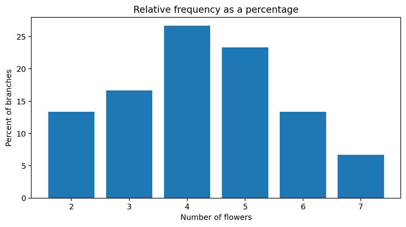
| Flowers | Frequency | Relative frequency | Percentage | Cumulative frequency |
|---|---|---|---|---|
| 2 | 4 | 0.133 | 13.3% | 4 |
| 3 | 5 | 0.167 | 16.7% | 9 |
| 4 | 8 | 0.267 | 26.7% | 17 |
| 5 | 7 | 0.233 | 23.3% | 24 |
| 6 | 4 | 0.133 | 13.3% | 28 |
| 7 | 2 | 0.067 | 6.7% | 30 |
Worked Example 2: Continuous Frequency Distribution
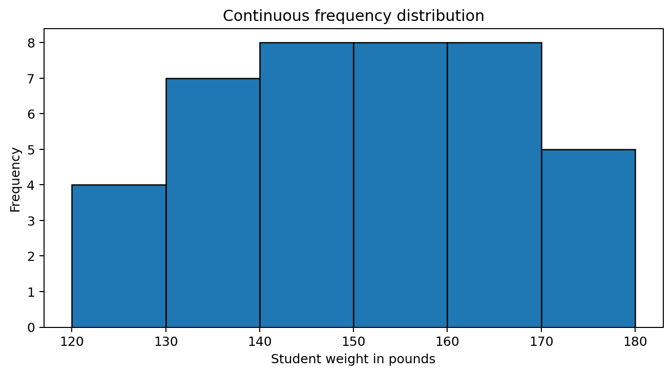
Problem. The weights of 40 students are measured in pounds. Weight is a continuous variable, so the values are grouped into class intervals.
Step 1. Minimum value = 121.5. Maximum value = 178.8.
Step 2. Range = 178.8 minus 121.5 = 57.3.
Step 3. Sturges formula gives m = 1 + 3.3 log 40 = 6.29, which is about 6 classes.
Step 4. Class interval = 57.3 divided by 6 = 9.55. A simple class interval of 10 pounds is used.
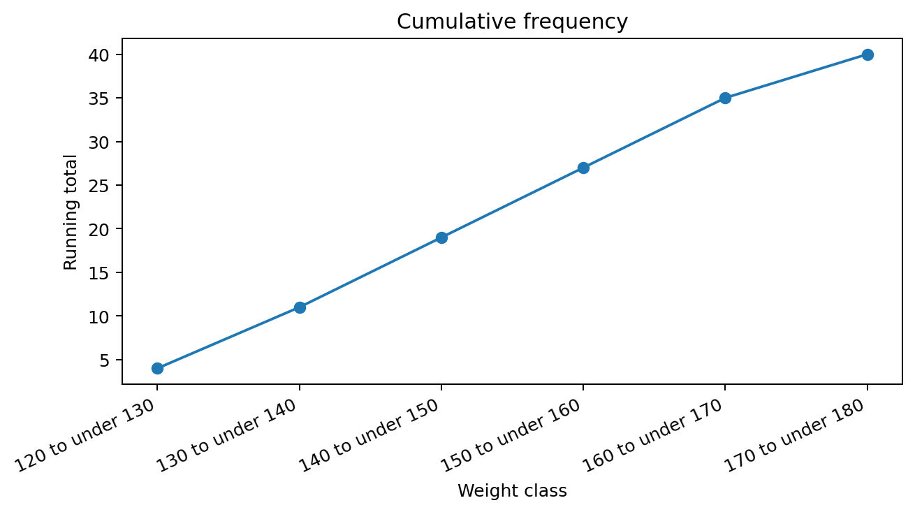
| Class interval | Mid value | Frequency | Cumulative frequency | Relative frequency | Percentage |
|---|---|---|---|---|---|
| 120 to under 130 | 125 | 4 | 4 | 0.100 | 10.0% |
| 130 to under 140 | 135 | 7 | 11 | 0.175 | 17.5% |
| 140 to under 150 | 145 | 8 | 19 | 0.200 | 20.0% |
| 150 to under 160 | 155 | 8 | 27 | 0.200 | 20.0% |
| 160 to under 170 | 165 | 8 | 35 | 0.200 | 20.0% |
| 170 to under 180 | 175 | 5 | 40 | 0.125 | 12.5% |
Animated cumulative frequency line
Cumulative frequency can only stay the same or increase because it is a running total.
Common mistake. Do not let class intervals overlap. A value should belong to one class only.
Worked Example 3: Bivariate Frequency Distribution
Problem. Twenty four students are classified by height group and weight group. This is a two way classification because two variables are used at the same time.
| Height group | 100 to under 120 | 120 to under 140 | 140 to under 160 | 160 to under 180 | Total |
|---|---|---|---|---|---|
| 60 to under 64 | 3 | 0 | 0 | 0 | 3 |
| 64 to under 68 | 0 | 7 | 1 | 0 | 8 |
| 68 to under 72 | 0 | 1 | 6 | 1 | 8 |
| 72 to under 76 | 0 | 0 | 0 | 5 | 5 |
| Total | 3 | 8 | 7 | 6 | 24 |
Chapter Summary
| Term | Meaning | Formula or note |
|---|---|---|
| Statistics | Methods used to collect, organize, present, analyze, and interpret numerical data | |
| Variable | A characteristic that takes numerical values | |
| Attribute | A quality or category that is described | |
| Continuous variable | A variable that can take any value within a range | |
| Discrete variable | A variable that takes separate countable values | |
| Primary data | Data collected first hand for the current study | |
| Secondary data | Data already collected for another purpose | |
| Classification | Arranging observations into similar groups | |
| Tabulation | Arranging data in rows and columns | |
| Frequency | Number of times a value or class occurs | |
| Range | Spread from smallest to largest value | Maximum minus minimum |
| Mid value | Center of a class interval | Upper plus lower, divided by 2 |
| Relative frequency | Share of total observations in a class | Class frequency divided by total frequency |
| Cumulative frequency | Running total of frequencies | |
| Bivariate distribution | Frequency table using two variables |
Common Mistakes
- Confusing a variable with an attribute.
- Calling count data continuous.
- Using secondary data without checking the source and definition.
- Building overlapping class intervals.
- Forgetting to check that total frequency equals the number of observations.
- Using Sturges formula as an exact rule rather than an approximate guide.
- Reading a statistical result without thinking about how the data were collected.
- Treating a group result as if it must describe every individual case.
Study Checklist
- I can explain statistics in both the plural and technical sense.
- I can list the main steps of the statistical method.
- I can explain the characteristics and limitations of statistics.
- I can tell variables from attributes.
- I can tell continuous variables from discrete variables.
- I can compare primary and secondary data.
- I can explain classification and tabulation.
- I can calculate range, class interval, and mid value.
- I can build discrete and continuous frequency tables.
- I can calculate relative frequency and cumulative frequency.
- I can read a two way frequency table.