
Least Squares Regression: Calculate the Regression Line Step by Step
Learn least squares regression step by step. Understand residuals, SSE, normal equations, slope, intercept, fitted regression lines, prediction
Least Squares Regression and Prediction: A Step by Step Guide
Quick answer: Least squares regression chooses the straight line that makes the total squared vertical errors as small as possible. Once the slope b and intercept a are known, the fitted line Ŷ = a + bX can be used to estimate Y for a selected X.
1. From the regression model to least squares
Lecture 1 introduced the population model Yi = α + βXi + εi. In a sample, α and β are unknown, so we estimate them with a and b. The sample relation is:
Yi = a + bXi + ei
The fitted value is the value on the estimated line:
Ŷi = a + bXi
Many lines can pass through the same scatter plot. The least squares method gives us a rule for choosing one. It selects the line that makes the total squared vertical differences between observed and fitted Y values as small as possible.
2. Observed Y, fitted Ŷ, and the residual
ei = Yi - Ŷi
A residual is positive when the observed point is above the fitted line. It is negative when the observed point is below the line. It is zero when the point is exactly on the line.
Interactive teaching visual. The vertical segments are residuals. A static image and data table are provided below.
| X | Observed Y | Fitted Ŷ | Residual e | e² |
|---|---|---|---|---|
| 5 | 16 | 15.625 | 0.375 | 0.1406 |
| 6 | 19 | 18.456 | 0.544 | 0.2959 |
| 8 | 23 | 24.118 | -1.118 | 1.2499 |
| 10 | 28 | 29.780 | -1.780 | 3.1684 |
| 12 | 36 | 35.442 | 0.558 | 0.3114 |
3. Why square the residuals?
If raw residuals are added, positive and negative values can cancel. Squaring makes every contribution nonnegative. It also gives more weight to larger misses.
S(a,b) = Σei² = Σ(Yi - a - bXi)²
Least squares chooses a and b to make this quantity as small as possible.
Current SSE:
Move the sliders. The least squares values are a = 1.47 and b = 2.831 for the rounded textbook equation.
| Candidate line | Equation | Sum of squared residuals |
|---|---|---|
| Least squares line | Ŷ = 1.47 + 2.831X | 15.89 |
| Candidate A | Ŷ = 5.00 + 2.500X | 33.00 |
| Candidate B | Ŷ = -3.00 + 3.200X | 37.32 |
4. Normal equations and direct formulas
Minimizing the squared residuals leads to two normal equations. They are solved together for a and b.
ΣY = na + bΣXΣXY = aΣX + bΣX²
For regression of Y on X, the direct slope formula is:
b = [nΣXY - (ΣX)(ΣY)] / [nΣX² - (ΣX)²]
Then find the intercept:
a = Ȳ - bX̄
The deviation form is also useful:
b = Σxy / Σx²where x = X - X̄ and y = Y - Ȳ.
The fitted line can be written as:
Ŷ = a + bXŶ = Ȳ + b(X - X̄)
The second form shows that the fitted line passes through (X̄, Ȳ).
5. Example 10.1, calculate the regression line step by step
The source provides nine X and Y pairs. We build XY and X² because these totals are needed for the slope formula.
| X | Y | XY | X² |
|---|---|---|---|
| 5 | 16 | 80 | 25 |
| 6 | 19 | 114 | 36 |
| 8 | 23 | 184 | 64 |
| 10 | 28 | 280 | 100 |
| 12 | 36 | 432 | 144 |
| 13 | 41 | 533 | 169 |
| 15 | 44 | 660 | 225 |
| 16 | 45 | 720 | 256 |
| 17 | 50 | 850 | 289 |
| Total = 102 | Total = 302 | Total = 3853 | Total = 1308 |
Step 1. Find the means
n = 9X̄ = 102 / 9 = 11.33Ȳ = 302 / 9 = 33.56
Step 2. Calculate b
b = [9(3853) - (102)(302)] / [9(1308) - (102)²]b = (34677 - 30804) / (11772 - 10404)b = 3873 / 1368 = 2.831
A one unit increase in X is associated with an estimated increase of about 2.831 units in Y.
Step 3. Calculate a
a = 33.56 - (2.831)(11.33) = 1.47
Step 4. Write the equation
Ŷ = 1.47 + 2.831X
Observed points appear first. The fitted line and mean point are then shown. The static data table above contains the same evidence.
6. Prediction with the fitted equation
Suppose we want a fitted prediction when X = 20.
Ŷ = 1.47 + 2.831(20)Ŷ = 58.09
The fitted value is about 58.09. A future observed Y value can differ because the regression line gives an estimate, not a guaranteed outcome.
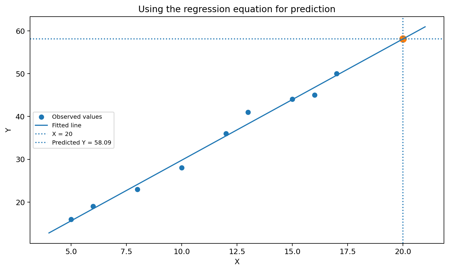
Prediction at X = 20.
7. Regression of Y on X versus regression of X on Y
Regression direction is part of the question. If Y is the prediction target, use regression of Y on X. If X is the prediction target, use regression of X on Y. The two fitted equations are usually different.
| Regression | Goal | Predicted variable | Predictor | Slope denominator | Error direction |
|---|---|---|---|---|---|
| Y on X | Predict Y from X | Y | X | nΣX² - (ΣX)² | Vertical Y differences |
| X on Y | Predict X from Y | X | Y | nΣY² - (ΣY)² | X direction differences |
Do not solve the first regression equation for X and treat that as the second regression. Each equation is fitted for its own prediction target.
8. Spring example, two prediction questions
The source spring experiment uses load X in pounds and spring length Y in inches.
| X | Y | X² | Y² | XY |
|---|---|---|---|---|
| 3 | 10 | 9 | 100 | 30 |
| 5 | 12 | 25 | 144 | 60 |
| 6 | 15 | 36 | 225 | 90 |
| 9 | 18 | 81 | 324 | 162 |
| 10 | 20 | 100 | 400 | 200 |
| 12 | 22 | 144 | 484 | 264 |
| 15 | 27 | 225 | 729 | 405 |
| 20 | 30 | 400 | 900 | 600 |
| 22 | 32 | 484 | 1024 | 704 |
| 28 | 34 | 784 | 1156 | 952 |
| 130 | 220 | 2288 | 5486 | 3467 |
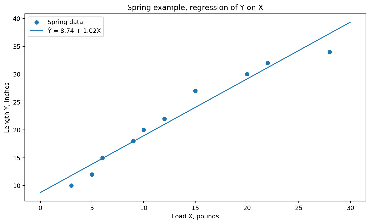
Predict Y from X
byx = 1.02ayx = 8.74Ŷ = 8.74 + 1.02X
Predict X from Y
bxy = 0.94axy = -7.68X̂ = -7.68 + 0.94Y
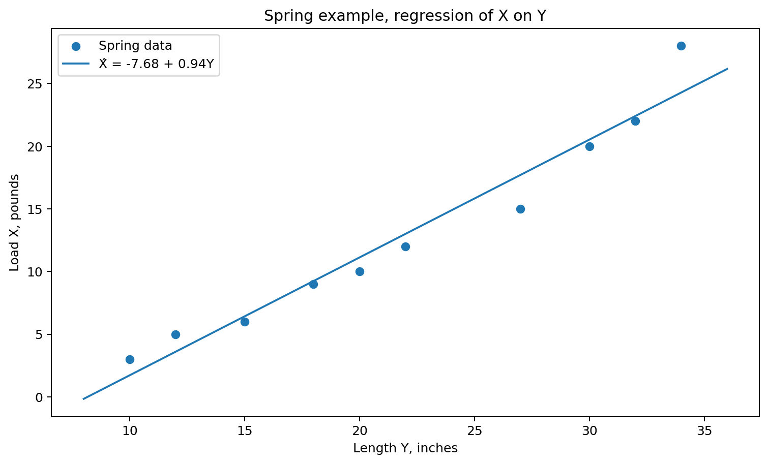
The first line predicts length from load. The second predicts load from length. Their slopes and intercepts differ because the fitting direction differs.
9. Properties of the least squares regression line
| Property | Formula or statement | What to remember |
|---|---|---|
| Passes through the means | The line passes through (X̄, Ȳ) | The sample mean point lies on the fitted line. |
| Residuals sum to zero | Σ(Y - Ŷ) = 0 | Small hand rounding can create a tiny difference. |
| Squared residuals are minimum | Σ(Y - Ŷ)² is minimized | This is the defining least squares property. |
| Line of best fit | Best under the least squares criterion | For Y on X, best means the smallest total squared vertical error. |
| Sample estimates | a estimates α, b estimates β | The sample equation estimates the population relation. |
10. Step by step regression calculation checklist
- Write the X and Y data.
- Add XY and X² columns.
- Find the totals.
- Write n.
- Calculate b.
- Find X̄ and Ȳ if needed.
- Calculate a.
- Write Ŷ = a + bX.
- Interpret b.
- Use the equation for prediction.
- Check that the line passes through the means.
11. Common mistakes
| Mistake | Correct approach |
|---|---|
| Treating Y and Ŷ as the same | Y is observed. Ŷ is fitted from the line. |
| Using the wrong residual sign | This lecture defines eᵢ = Yᵢ - Ŷᵢ. |
| Adding residuals instead of squared residuals | Raw positive and negative residuals can cancel. |
| Forgetting n in the direct slope formula | The numerator and denominator both use n. |
| Using ΣY² in the denominator for Y on X | Y on X uses nΣX² - (ΣX)². |
| Using ΣX² in the denominator for X on Y | X on Y uses nΣY² - (ΣY)². |
| Rounding too early | Keep several decimals until the final answer. |
| Treating a prediction as a certain outcome | A fitted value is an estimate, not a guaranteed observation. |
12. Formula revision table
| Concept | Formula |
|---|---|
| Residual | eᵢ = Yᵢ - Ŷᵢ |
| Least squares objective | S(a,b) = Σ(Yᵢ - a - bXᵢ)² |
| First normal equation | ΣY = na + bΣX |
| Second normal equation | ΣXY = aΣX + bΣX² |
| Slope for Y on X | b = [nΣXY - (ΣX)(ΣY)] / [nΣX² - (ΣX)²] |
| Intercept | a = Ȳ - bX̄ |
| Fitted line | Ŷ = a + bX |
| Mean form | Ŷ = Ȳ + b(X - X̄) |
| Slope for X on Y | b_xy = [nΣXY - (ΣX)(ΣY)] / [nΣY² - (ΣY)²] |
| X on Y line | X̂ = a_xy + b_xyY |
FAQs
1. What is the principle of least squares?
The principle of least squares chooses the regression line that makes the total squared residuals as small as possible. In other words, it minimizes:
∑ei2
where each residual is the difference between the observed value and the fitted value.
2. What is a residual in regression?
A residual measures how far an observed value is from the value predicted by the regression line.
ei=Yi−Y^i
A positive residual means the observed value is above the fitted line. A negative residual means it is below the line.
3. What is the estimated regression equation?
The estimated simple linear regression equation is:
Y^=a+bX
Here, a is the intercept and b is the slope or regression coefficient. The equation is used to estimate or predict Y for a given value of X.
4. What does the slope b mean in a regression equation?
The slope b shows the estimated change in Y when X increases by one unit.
If b is positive, Y tends to increase as X increases. If b is negative, Y tends to decrease as X increases.
5. Why are regression of Y on X and regression of X on Y different?
Regression of Y on X is used when we want to predict Y from X. Regression of X on Y is used when we want to predict X from Y.
The two regression lines are generally different because each one minimizes errors in a different direction. The spring example in the chapter shows this clearly.