
Linear Regression Calculator With Intervals and Plots
This linear regression calculator fits a straight line to paired X and Y values. It returns the regression equation, slope, intercept, correlation, R squared, coefficient details, an ANOVA summary, and error measures.…
Linear Regression Calculator With Intervals and Plots
A linear regression calculator fits a straight line to paired numeric data. It can estimate the slope and intercept, measure the strength of the linear relationship, test whether the slope differs from zero, predict a new response, and show uncertainty around that prediction.
The quickest way to use one is simple. Enter matching X and Y values, choose a confidence level, add a new X value if you want a prediction, then read the fitted equation and the interval results. After that, check the plots. A strong R squared value can look impressive, but the model still needs sensible residuals and a reasonable data range.
This guide uses one synthetic study hours and exam score dataset from start to finish. The numbers are teaching data, not results from a real study. That makes it possible to verify every table, interval, and plot from the same ten observations.
Quick example input
| Study hours X | Exam score Y |
|---|---|
| 1 | 52 |
| 2 | 55 |
| 3 | 61 |
| 4 | 64 |
| 5 | 66 |
In this guide
- What the Calculator Does and When Linear Regression Fits
- Enter Data, Pick Variables, and Set the Calculation Options
- How Least Squares Finds the Regression Equation
- Read the Regression Results Without Guessing
- Confidence Intervals and Prediction Intervals
- Use Plots and Diagnostics to Check the Model
- Worked Example From Raw Data to a Predicted Value
- Assumptions, Alternatives, Reporting, and FAQs
What the Calculator Does and When Linear Regression Fits
Simple linear regression studies the relationship between one numeric predictor and one numeric response. The predictor is often called X. The response is often called Y. The calculator finds the straight line that best summarizes how Y tends to change as X changes.
The fitted value is the Y value predicted by the line. A residual is the observed Y value minus that fitted value. Residuals matter because they show what the line did not explain. Small, pattern free residuals are a good sign. Clear structure in the residuals is a warning that the straight line may be missing something important.
Good reasons to use simple linear regression
- Estimate how much Y changes, on average, when X rises by one unit.
- Describe the strength and direction of a linear association.
- Test whether the population slope is likely to differ from zero.
- Estimate the mean response for a chosen X value.
- Predict one new response for a chosen X value, with a prediction interval.
Regression describes association. By itself, it does not prove that changing X causes Y to change. Causal claims need a suitable study design and supporting evidence beyond a fitted line.
Table 1. Choosing a regression method
| Method | Use it when | Typical outcome | Main caution |
|---|---|---|---|
| Simple linear regression | One numeric predictor is used to explain one numeric response | Numeric Y | The relationship should be reasonably linear |
| Multiple linear regression | Several predictors are needed at the same time | Numeric Y | Predictors can overlap in what they explain |
| Logistic regression | The response is a category such as yes or no | Category or probability | A straight line model for numeric Y is not appropriate |
| Polynomial regression | The response follows a clear curve that a polynomial can describe | Numeric Y | Higher order terms can overfit and extrapolate badly |
Enter Data, Pick Variables, and Set the Calculation Options
A calculator needs paired observations. Each X value must belong to the Y value in the same row. If a student studied four hours and scored 64, those two values form one pair. Changing the row order of one column without changing the other destroys the pairing and changes the analysis.
Calculator quick start
- Paste or type the X values in the predictor column.
- Paste or type the matching Y values in the response column.
- Give each variable a short label with a unit when a unit exists.
- Choose a confidence level, commonly 95 percent.
- Enter a new X value if you want a fitted value and interval estimates.
- Run the calculation, then read the results and inspect the plots before drawing a conclusion.
Table 2. Calculator inputs and validation rules
| Input | What to enter | Validation rule |
|---|---|---|
| X values | Numeric predictor values | Must include variation. A constant X cannot define a slope |
| Y values | Numeric response values paired row by row with X | Usable X and Y counts must match |
| Variable labels | Clear names such as study hours and exam score | Use labels that make the output easy to read |
| Confidence level | A supported level such as 90, 95, or 99 percent | Use the same level for all intervals you compare |
| Prediction X | One or more X values where a prediction is needed | Prefer values within the observed X range |
| Missing entries | Blank or missing values that are reviewed before analysis | Do not turn missing values into zero without evidence |
What to do with outliers and duplicate X values
Duplicate X values can be valid because different observations can share the same predictor value. An unusual point also should not be removed just because it weakens the fit. Check whether it is a data error, a valid rare case, or an influential observation. If you report results with and without a point, explain the reason and show both results clearly.
How Least Squares Finds the Regression Equation
The fitted line is written as predicted Y equals the intercept plus the slope times X. The slope tells you how much the fitted Y changes when X increases by one unit. The intercept is the fitted Y value when X equals zero.
ŷ = b₀ + b₁x
Ordinary least squares chooses the slope and intercept that make the sum of squared residuals as small as possible. Squaring gives large misses more weight and prevents positive and negative residuals from canceling each other.
b₁ = Σ[(xᵢ − x̄)(yᵢ − ȳ)] ÷ Σ[(xᵢ − x̄)²]b₀ = ȳ − b₁x̄eᵢ = yᵢ − ŷᵢ
Here, x̄ is the mean of X, ȳ is the mean of Y, b₁ is the sample slope, b₀ is the sample intercept, and eᵢ is the residual for observation i. Software does this arithmetic quickly, but the formulas show what the calculator is optimizing.
Table 3. Worked least squares calculation values
| X | Y | Fitted Y | Residual | Squared residual |
|---|---|---|---|---|
| 1 | 52 | 51.87 | 0.13 | 0.016 |
| 2 | 55 | 55.75 | −0.75 | 0.556 |
| 3 | 61 | 59.62 | 1.38 | 1.909 |
| 4 | 64 | 63.49 | 0.51 | 0.259 |
| 5 | 66 | 67.36 | −1.36 | 1.860 |
| 6 | 72 | 71.24 | 0.76 | 0.583 |
| 7 | 74 | 75.11 | −1.11 | 1.230 |
| 8 | 79 | 78.98 | 0.02 | 0.000 |
| 9 | 82 | 82.85 | −0.85 | 0.730 |
| 10 | 88 | 86.73 | 1.27 | 1.620 |
For these ten pairs, the fitted equation is ŷ = 48.00 + 3.8727x. The slope is positive, so higher study hours are associated with higher fitted exam scores in this synthetic sample.
Read the Regression Results Without Guessing
A useful calculator should report more than a line. The slope and intercept describe the fitted equation. R and R squared describe linear association and explained sample variation. Standard errors and test statistics describe sampling uncertainty. Residual measures describe how far the observations sit from the fitted line.
Table 4. Regression output and plain English meaning
| Statistic | Illustrative value | What it means | Common mistake |
|---|---|---|---|
| Sample size | 10 | Ten paired observations were used | A larger sample does not fix poor measurement or bad design |
| Intercept | 48.00 | Fitted exam score when study hours equal zero | Do not force a practical meaning if zero is outside the useful data range |
| Slope | 3.8727 | Estimated score change for one more study hour | Do not call the slope a causal effect from regression alone |
| Correlation R | 0.9965 | Very strong positive linear association in this sample | R does not test every model assumption |
| R squared | 0.9930 | About 99.3 percent of sample Y variation is explained by the fitted line | A high value does not prove causation or guarantee good predictions |
| Residual standard error | 1.047 | Typical vertical residual size in exam score units | Do not confuse it with the slope standard error |
| Slope standard error | 0.1152 | Estimated sampling uncertainty of the slope | It is not the typical prediction error |
| Slope t statistic | 33.61 | Slope divided by its standard error | A large t value does not establish cause |
| Slope p value | 6.71 × 10⁻¹⁰ | Strong evidence against a zero slope under the model assumptions | A small p value does not measure practical importance |
| Slope 95 percent interval | 3.607 to 4.138 | Plausible values for the population slope under the model | Do not treat the interval as a range containing 95 percent of individual outcomes |
| F statistic | 1129.52 | Overall one predictor regression test | In simple regression it addresses the same slope relationship as the slope t test |
How to interpret the slope and intercept
The slope of 3.8727 means that each additional study hour is associated with an estimated 3.87 point increase in the fitted exam score. The intercept is 48.00. It is mathematically required for the line, but its practical value depends on whether zero study hours is a meaningful point for the question.
R squared is useful, but it is not a quality certificate
R squared measures the share of sample variation in Y explained by the fitted line. It does not show whether the relationship is causal, whether the data were collected well, whether errors are independent, or whether a curved pattern is hiding in the residuals. Those questions need design knowledge and diagnostic checks.
In simple linear regression with one predictor, the slope t test and the overall F test evaluate the same basic null hypothesis about the linear relationship. Adjusted R squared can also be reported, but it adds little in a one predictor model because there is only one explanatory variable to penalize.
Confidence Intervals and Prediction Intervals
A confidence interval for the mean response and a prediction interval for one new response answer different questions. The confidence interval estimates the average Y value for all cases with a chosen X. The prediction interval estimates where one new individual Y value may fall at that same X.
The prediction interval is wider because it includes uncertainty in the fitted mean plus the natural variation of individual outcomes around that mean. The two intervals should never be treated as interchangeable.
Mean response standard error = s × √[1 ÷ n + (x₀ − x̄)² ÷ Sxx]New response standard error = s × √[1 + 1 ÷ n + (x₀ − x̄)² ÷ Sxx]
In these formulas, s is the residual standard error, n is the sample size, x₀ is the chosen prediction value, x̄ is the mean X value, and Sxx is the sum of squared X deviations from the mean. The extra 1 inside the prediction formula accounts for individual outcome variation.
Table 5. Prediction at X = 7.5
| Prediction X | Fitted Y | Lower confidence limit | Upper confidence limit | Lower prediction limit | Upper prediction limit |
|---|---|---|---|---|---|
| 7.5 | 77.05 | 76.12 | 77.98 | 74.46 | 79.63 |
At 7.5 study hours, the fitted score is 77.05. The 95 percent confidence interval for the mean response is 76.12 to 77.98. The 95 percent prediction interval for one new score is 74.46 to 79.63. The prediction interval is wider, as it should be.
Why intervals widen away from the center
A fitted line is estimated most precisely near the center of the observed X values. As the chosen X moves toward the edge of the data, and especially beyond it, uncertainty grows. That is one reason extrapolation can be risky. A line that works well from one to ten study hours may not describe what happens at twenty hours.
Use Plots and Diagnostics to Check the Model
The regression equation is only part of the answer. Diagnostic plots help you decide whether a straight line is a reasonable summary of the data. NIST recommends examining residuals because patterns in them can reveal model structure that the fitted line failed to capture.
Scatter plot with fit and uncertainty bands
The points follow a strong upward linear pattern. The confidence band stays close to the fitted line because the sample relationship is very tight. The prediction band is wider because one future score can vary around the mean response even when the mean is estimated precisely.
Residuals versus fitted values
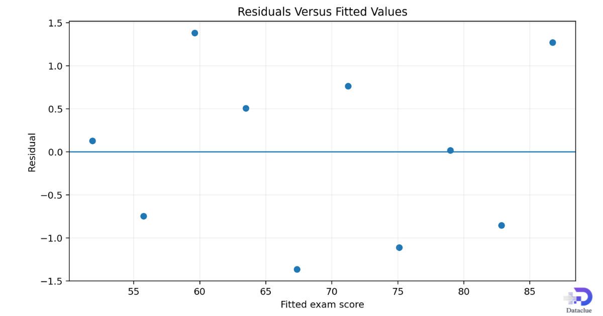
A healthy residual plot usually looks like a random cloud around zero with a fairly even vertical spread. Curvature can suggest that the straight line is missing a nonlinear pattern. A funnel shape can suggest changing variance. Clusters can point to groups that should be modeled or studied separately.
Normal Q Q plot
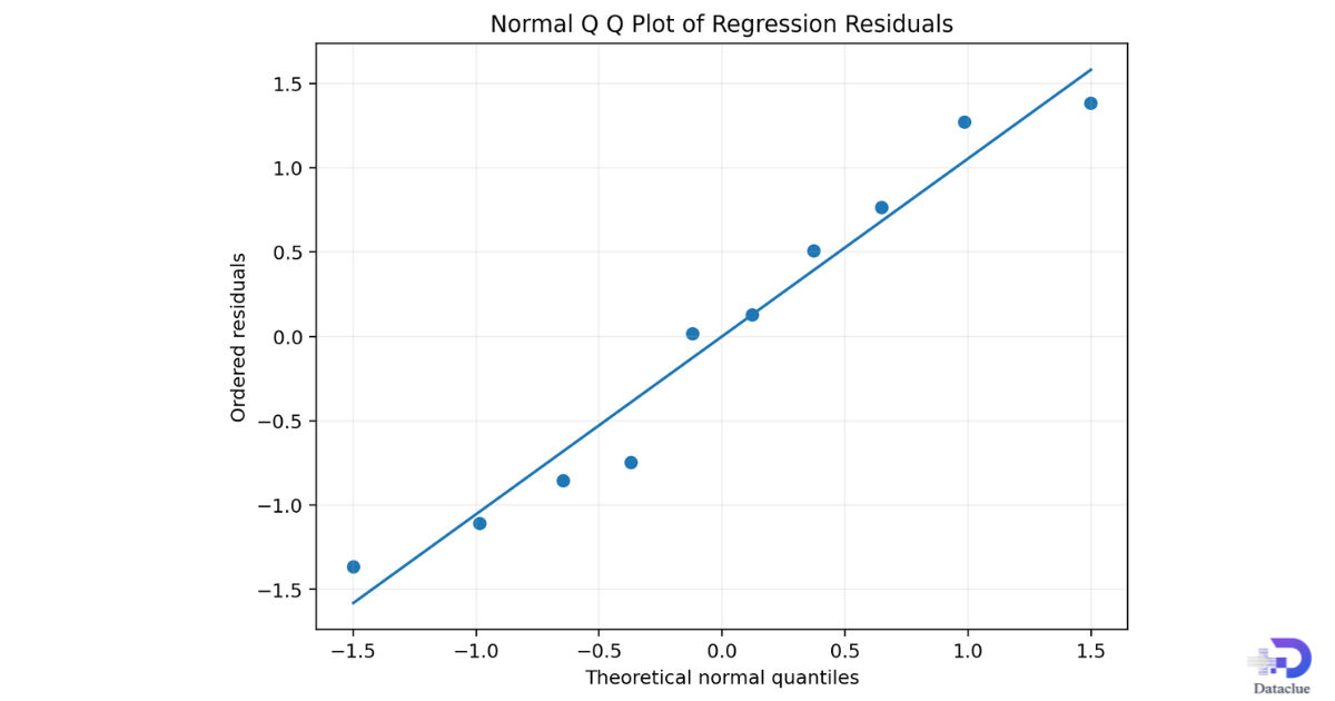
A Q Q plot compares the ordered residuals with values expected from a normal distribution. Points that stay reasonably close to the reference line support the normal residual assumption. Strong bends, extreme tail departures, or isolated points deserve closer review, especially in a small sample.
Independence and influential observations
Independence is not visible in every scatter plot. If observations were collected over time, by location, or in repeated groups, the order and study design matter. A residual plot against time or sequence can reveal dependence that a residuals versus fitted plot may miss.
An observation with a large residual is unusual in Y, but influence also depends on where its X value sits and how strongly it changes the fitted line. Do not delete a point only because it makes R squared smaller. Check the data record, the study process, and the effect of the point on the conclusions.
Worked Example From Raw Data to a Predicted Value
The full example uses ten synthetic observations. X is study hours and Y is exam score. The data were created only to demonstrate the calculations. They should not be treated as evidence about real students.
Table 6. Synthetic data used throughout the article
| Study hours X | Exam score Y |
|---|---|
| 1 | 52 |
| 2 | 55 |
| 3 | 61 |
| 4 | 64 |
| 5 | 66 |
| 6 | 72 |
| 7 | 74 |
| 8 | 79 |
| 9 | 82 |
| 10 | 88 |
Step 1: Fit the line
The least squares calculation gives ŷ = 48.00 + 3.8727x. The fitted line rises by about 3.87 exam score points for each additional study hour in this sample.
Step 2: Measure fit and test the slope
The correlation is 0.9965 and R squared is 0.9930. The residual standard error is 1.047 score points. The slope t statistic is 33.61, with a very small p value. Under the regression assumptions, the data provide strong evidence of a positive linear association. This result does not prove that extra study time causes the score increase.
Step 3: Predict at 7.5 study hours
At X = 7.5, the fitted exam score is 77.05. The 95 percent confidence interval for the mean response is 76.12 to 77.98. The 95 percent prediction interval for one new student score is 74.46 to 79.63.
Step 4: Check diagnostics before trusting the story
The residual plot does not show a strong curve or obvious funnel in this small synthetic example. The Q Q plot is also reasonably close to a straight pattern. That supports using the simple linear model for teaching here, but a real analysis would also check study design, measurement quality, independence, and influential cases.
Assumptions, Alternatives, Reporting, and FAQs
A regression calculator can produce numbers even when the model is a poor choice. The final step is to connect the assumptions, the plots, and the research question.
Table 7. Regression assumptions, warning signs, and possible actions
| Assumption or condition | What to check | Warning sign | Possible response |
|---|---|---|---|
| Linearity | Scatter plot and residual pattern | Clear curve | Try a justified transformation or polynomial form |
| Independent errors | Study design and residuals in collection order | Runs, cycles, or time pattern | Use a model that accounts for dependence |
| Constant variance | Residual spread across fitted values | Funnel shape | Consider a transformation or weighted least squares |
| Approximate residual normality | Q Q plot and supporting histogram | Strong tail departures | Review outliers, sample size, and robust methods |
| Appropriate numeric variables | Meaning and scale of X and Y | Categorical Y or badly coded values | Choose a model that matches the outcome type |
| No harmful extrapolation | Prediction X compared with observed range | Prediction far beyond the data | Collect data in the needed range or avoid the prediction |
What to use when simple linear regression is not enough
A clear curve may call for polynomial regression or another nonlinear form. Strong influence from unusual points may justify a robust regression method after the observations are checked. Changing residual variance may point to weighted least squares or a transformation. Several important predictors may require multiple linear regression. A categorical response, such as yes or no, calls for logistic regression instead of simple linear regression.
Ridge, lasso, and partial least squares are advanced options for predictor problems such as many correlated variables. They solve different problems from a basic one predictor calculator, so they should not be treated as simple replacements for ordinary least squares.
Verify the result in Python
import numpy as np
from scipy import stats

x = np.arange(1, 11, dtype=float)
y = np.array([52, 55, 61, 64, 66, 72, 74, 79, 82, 88], dtype=float)

result = stats.linregress(x, y)
print(result.slope, result.intercept, result.rvalue ** 2, result.pvalue)
Verify the result in R
x <- 1:10
y <- c(52, 55, 61, 64, 66, 72, 74, 79, 82, 88)
model <- lm(y ~ x)
summary(model)
confint(model)
predict(model, data.frame(x = 7.5), interval = "confidence")
predict(model, data.frame(x = 7.5), interval = "prediction")
Simple reporting template
A simple linear regression of exam score on study hours gave the fitted equation ŷ = 48.00 + 3.8727x, with R squared = 0.9930 and n = 10. The estimated slope was 3.8727, 95 percent confidence interval 3.607 to 4.138, t(8) = 33.61, p < 0.001. At 7.5 study hours, the fitted score was 77.05, with a 95 percent prediction interval from 74.46 to 79.63.
Frequently asked questions
What is the difference between correlation and regression?
Correlation summarizes the strength and direction of a linear association. Regression also gives an equation that predicts or estimates Y from X.
What does R squared mean?
R squared is the share of sample variation in Y explained by the fitted regression line. It does not prove causation and it does not replace diagnostic checks.
Why is the prediction interval wider than the confidence interval?
The prediction interval includes uncertainty in the fitted mean plus the natural variation of one individual outcome. The mean response confidence interval does not include that extra individual variation.
Can I predict outside the observed X range?
You can calculate a number, but the result may be unreliable because the straight line may not continue beyond the data. Extrapolate only with strong subject knowledge and clear limits.
Should I remove an outlier?
Not automatically. First check whether the point is a data error, a valid unusual case, or an influential observation. Report any justified exclusion clearly.
Is a small p value enough to trust the model?
No. A small p value addresses evidence about the slope under the model. You still need to check linearity, residual behavior, independence, measurement quality, and practical importance.
When should I use multiple regression instead?
Use multiple regression when several predictors are needed to answer the question and the data support estimating their effects together.
Sources and method note
The statistical interpretation in this guide follows standard simple linear regression material from Penn State STAT 501 and residual checking guidance from the NIST Engineering Statistics Handbook. The worked data are synthetic. All fitted values, tests, intervals, and plots in this article were calculated from the ten pairs shown in Table 6.
- Penn State STAT 501: Simple Linear Regression
- Penn State STAT 501: Model Evaluation
- Penn State STAT 501: Estimation and Prediction
- NIST Engineering Statistics Handbook: Check of Assumptions
- Google Search Central: Creating Helpful, Reliable, People First Content
- Google Search Central: Guide to Generative AI Features on Search
Try it in DataClue
Ready to run Simple Linear Regression?
Fit a simple regression model with one numeric predictor (X) and one numeric outcome (Y) using OLS.
Run Simple Linear Regression