
Machine Learning for Economic Forecasting: What Works?
Forecasting and Machine Learning
Machine Learning for Economic Forecasting: What Works?
A U.S. pillar guide with FRED data, real model results, time ordered validation, nowcasting, and failure analysis.
Machine learning can improve economic forecasts, but it does not win by default. In U.S. macro data, simple baselines are hard to beat because the sample is small, the data are revised, and the economy changes when shocks arrive. The best first choice is often a regularized linear model such as Ridge or Elastic Net. Tree models can help when there are real nonlinear patterns and enough data, but they can fail when the future moves outside the range seen in training. Ensembles can improve stability. Neural networks need a strong reason and enough observations.
Contents
- The short answer: what works?
- Why this matters in the U.S. economy now
- What economic forecasting means
- Why machine learning is attractive
- Why economic data are unusually hard
- A practical FRED data stack
- A simple Python starting point
- The fair test comes before the fancy model
- Our reproducible U.S. inflation model comparison
- What the inflation test teaches
- What research says about simple versus complex models
- Model families: when each one makes sense
- GDP forecasting: machine learning is often a nowcasting problem
- Inflation forecasting: persistence makes the baseline strong
- Unemployment forecasting: watch the leading labor signals
- Recession prediction: the rare event problem
- Nowcasting versus forecasting
- How to evaluate a model fairly
- Real time data and vintage data are not optional details
- Interpretability: useful, but not causality
- A production workflow that survives contact with new data
- Decision framework: which model should you try first?
- Google Search standards for publishing this research
- Limitations
- Conclusion
The short answer: what works?
For economic forecasting machine learning, the model name matters less than the testing design. Start with a forecast that is hard to embarrass. For inflation, that may be last month's rate. For unemployment, it may be a simple autoregression. For GDP, it may be a bridge model or a factor model. Then ask whether the machine learning model improves the same future dates with the same information.
Across research and our own U.S. inflation test, four lessons repeat. First, regularized linear models are strong when the number of observations is limited. Second, tree based models are useful for nonlinear patterns but weak at extrapolation. Third, forecast combinations can reduce the damage from a single bad model. Fourth, random cross validation is a poor choice for most macro time series because it lets the model learn from a future that would not have existed at the forecast date.
That is the practical answer to what works. Use the simplest model that earns its complexity in a fair out of sample test.
Why this matters in the U.S. economy now
Forecasting is not a classroom exercise. The U.S. data are moving in different directions, which is exactly when model discipline matters. In July 2026, headline CPI was 3.4 percent higher than a year earlier and core CPI was up 2.5 percent. The unemployment rate was 4.1 percent. Real GDP grew at a 1.5 percent annual rate in the second quarter second estimate released August 26. The Atlanta Fed GDPNow estimate for third quarter 2026 growth was about 4.61 percent on August 26, while the St. Louis Fed Economic News Index was about 1.93 percent on August 21. The gap between those nowcasts is a useful reminder that models can disagree even when they use current U.S. data.
Those numbers describe different parts of the economy and they arrive on different schedules. A model that treats every value as if it was known at the same time will look better on paper than it could have performed in real life. Good forecasting starts with the information calendar, not with the algorithm.
| Current U.S. signal | Latest value used here | Source date | Why a forecaster cares |
|---|---|---|---|
| Headline CPI | 3.4 percent year over year | July 2026 | Inflation target and price pressure |
| Core CPI | 2.5 percent year over year | July 2026 | Underlying inflation trend |
| Unemployment rate | 4.1 percent | July 2026 | Labor market slack and recession risk |
| Real GDP | 1.5 percent annual rate | Second quarter 2026 second estimate, August 26 | Broad output growth |
| Atlanta Fed GDPNow | 4.61 percent annual rate | Third quarter 2026, updated August 26 | Real time model estimate before official GDP |
| St. Louis Fed GDP nowcast | 1.93 percent annual rate | Third quarter 2026, updated August 21 | Second real time estimate that shows model disagreement |
What economic forecasting means
A forecast estimates a value that has not happened yet. A nowcast estimates the present before the official number is published. The difference is easy to miss, but it changes the model design.
A one month inflation forecast might use July data to predict August inflation. A GDP nowcast might use July retail sales, industrial production, housing, and labor data to estimate the third quarter while the quarter is still in progress. A six month unemployment forecast asks a harder question because the model must reach farther beyond the data it can see.
Every forecast should state four things clearly: the target, the forecast horizon, the information date, and the scoring rule. Without those four items, model comparisons are hard to trust.
Why machine learning is attractive
Economic data can contain many signals at once. Interest rates can interact with housing. Energy can affect inflation and consumer budgets. Credit conditions can matter more when firms are already weak. Machine learning can search for patterns across many variables without forcing every relationship to be a straight line.
Regularization is one reason machine learning can help even when the model is simple. Ridge and Elastic Net shrink unstable coefficients. That is useful when many economic series move together. Tree methods can split the data into different regions, so they can capture thresholds and interactions. Ensembles combine forecasts so one model does not control the whole result.
The attraction is real. The problem is that U.S. macro data do not look like a giant image or language data set. Monthly data since 1990 give only a few hundred observations. Quarterly GDP gives even fewer. A model with thousands of flexible choices can learn the past too closely.
Why economic data are unusually hard
Macroeconomic forecasting has several traps that are less severe in many other machine learning tasks.
- Small samples. Quarterly data produce very few independent observations by machine learning standards.
- Revisions. GDP, payrolls, seasonal factors, and other series can change after the first release.
- Publication lags. A July value may not be known until August or September.
- Structural breaks. A pandemic, financial crisis, energy shock, or policy change can alter old relationships.
- Rare events. The United States has only a limited number of modern recession episodes, which makes recession classification difficult.
- Strong persistence. Simple forecasts are often good because many macro variables move slowly.
- Common trends. Many predictors rise or fall together, which can make feature importance unstable.
A practical FRED data stack
FRED is a useful distribution layer because it brings together series from BLS, BEA, the Federal Reserve, Census, and other agencies. The series ID should be stored with the model code so another analyst can rebuild the feature set.
Do not treat a FRED download as proof that the timing is safe. Record the release date and the vintage. FRED and ALFRED support real time periods and vintage dates. That lets a strict backtest ask what value was actually available on a past forecast date.
| Forecast topic | Useful FRED series | Series ID | Typical role |
|---|---|---|---|
| Headline inflation | CPI, all urban consumers | CPIAUCSL | Target or price feature |
| Core inflation | CPI less food and energy | CPILFESL | Underlying price feature |
| Unemployment | Unemployment rate | UNRATE | Labor target or predictor |
| Payrolls | All employees, total nonfarm | PAYEMS | Labor momentum |
| Industry | Industrial production index | INDPRO | Real activity |
| Policy rate | Effective federal funds rate | FEDFUNDS | Monetary policy |
| Housing | Housing starts | HOUST | Rate sensitive demand |
| Retail demand | Advance retail and food services sales | RSAFS | Consumer activity |
| Yield curve | 10 year minus 2 year Treasury spread | T10Y2Y | Financial and recession signal |
| Recession labels | NBER recession indicator | USRECD | Classification target or evaluation label |
A simple Python starting point
The code below shows the shape of a basic FRED workflow. A production system should also save the download date, source notes, and vintage information.
import pandas as pd

def fred_series(series_id):
    url = "https://fred.stlouisfed.org/graph/fredgraph.csv?id=" + series_id
    data = pd.read_csv(url, parse_dates=["DATE"])
    return data.set_index("DATE")[series_id]

cpi = fred_series("CPIAUCSL")
unrate = fred_series("UNRATE")
indpro = fred_series("INDPRO")

features = pd.concat([cpi, unrate, indpro], axis=1)
features.columns = ["cpi", "unrate", "indpro"]
features["cpi_yoy"] = features["cpi"].pct_change(12) * 100
features["target_next_month"] = features["cpi_yoy"].shift(-1)
The fair test comes before the fancy model
The strongest forecasting article, notebook, or production system should make the test harder to game. The final test dates must stay untouched until model choices are finished. Every model must predict the same target dates. Features must use only information that existed at the forecast date.
For time series, use an expanding window or rolling window. Train on the past, predict the next period, move forward, and repeat. This is slower than one random split, but it matches how forecasting actually works.
Federal Reserve research on U.S. recession forecasting shows why this matters. In one study, ordinary random style cross validation made tree models look strongest. A more conservative time series procedure reversed the ranking and favored a simple probit model. The lesson is bigger than recession models. A weak validation design can change the winner.
- Set the target and horizon before model tuning.
- Keep the last period as a true holdout.
- Use only past information for each forecast.
- Tune hyperparameters on a validation period, not on the final holdout.
- Score the naive baseline first.
- Archive every forecast so weak periods cannot be removed later.
Our reproducible U.S. inflation model comparison
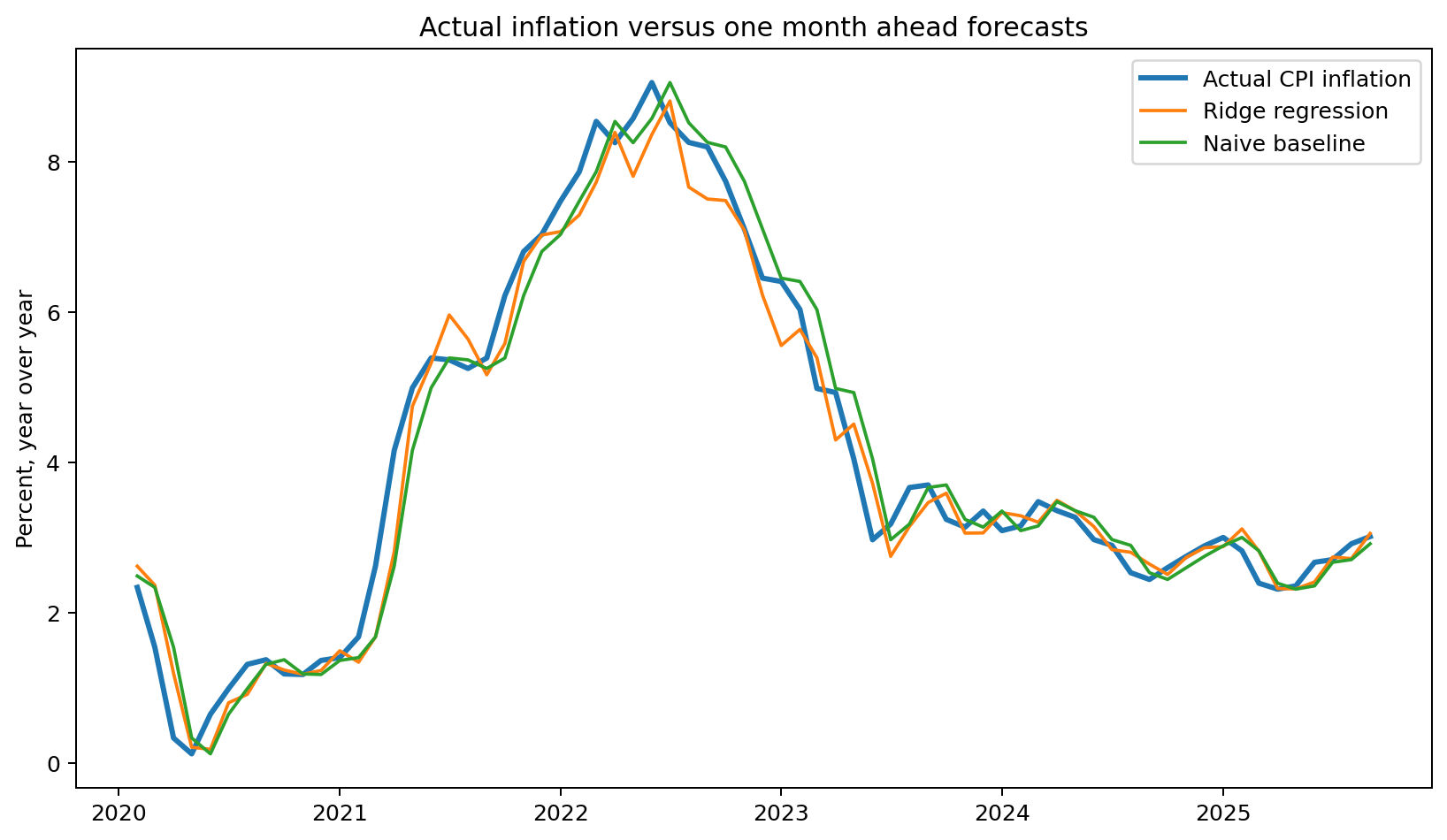
A companion test gives a concrete example. We predicted one month ahead U.S. CPI inflation. The target was the official year over year CPI rate. The training sample ran from January 1999 through December 2016 after lag construction. The validation period ran from January 2017 through December 2019. The final target holdout ran from February 2020 through September 2025.
The feature set used headline CPI, core CPI, energy, food, shelter, rent, and owners equivalent rent. We calculated annual and monthly changes, then added recent lags and rolling averages. Every model saw the same target months. No random shuffle was used.
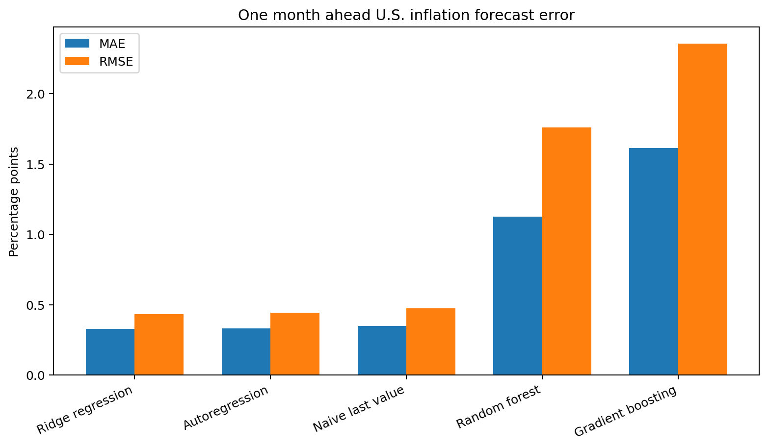
Ridge regression was the best model, but the win was small. Its mean absolute error was 0.327 percentage points. A basic autoregression reached 0.332. The naive last value forecast was 0.350. Random forest and gradient boosting were much worse because they struggled when inflation moved far beyond the range seen before the shock.
| Model | MAE | RMSE | Change in MAE versus naive | Reading |
|---|---|---|---|---|
| Ridge regression | 0.327 | 0.432 | 6.4 percent better | Best in this test |
| Autoregression | 0.332 | 0.444 | 5.1 percent better | Nearly tied with Ridge |
| Naive last value | 0.350 | 0.474 | Reference | Strong baseline |
| Random forest | 1.125 | 1.761 | 221.7 percent worse | Failed during shock |
| Gradient boosting | 1.614 | 2.355 | 361.3 percent worse | Failed more severely |
What the inflation test teaches
The result does not prove that Ridge is the best inflation model forever. It shows a more useful point. Complexity must earn its place.
The tree models learned useful shapes in the training data, but inflation after 2020 rose to levels they had not seen. Trees usually predict by averaging outcomes inside learned regions. They are not natural extrapolators. Ridge is still a linear model, so it can extend a relationship beyond the exact training range. That helped during the inflation surge.
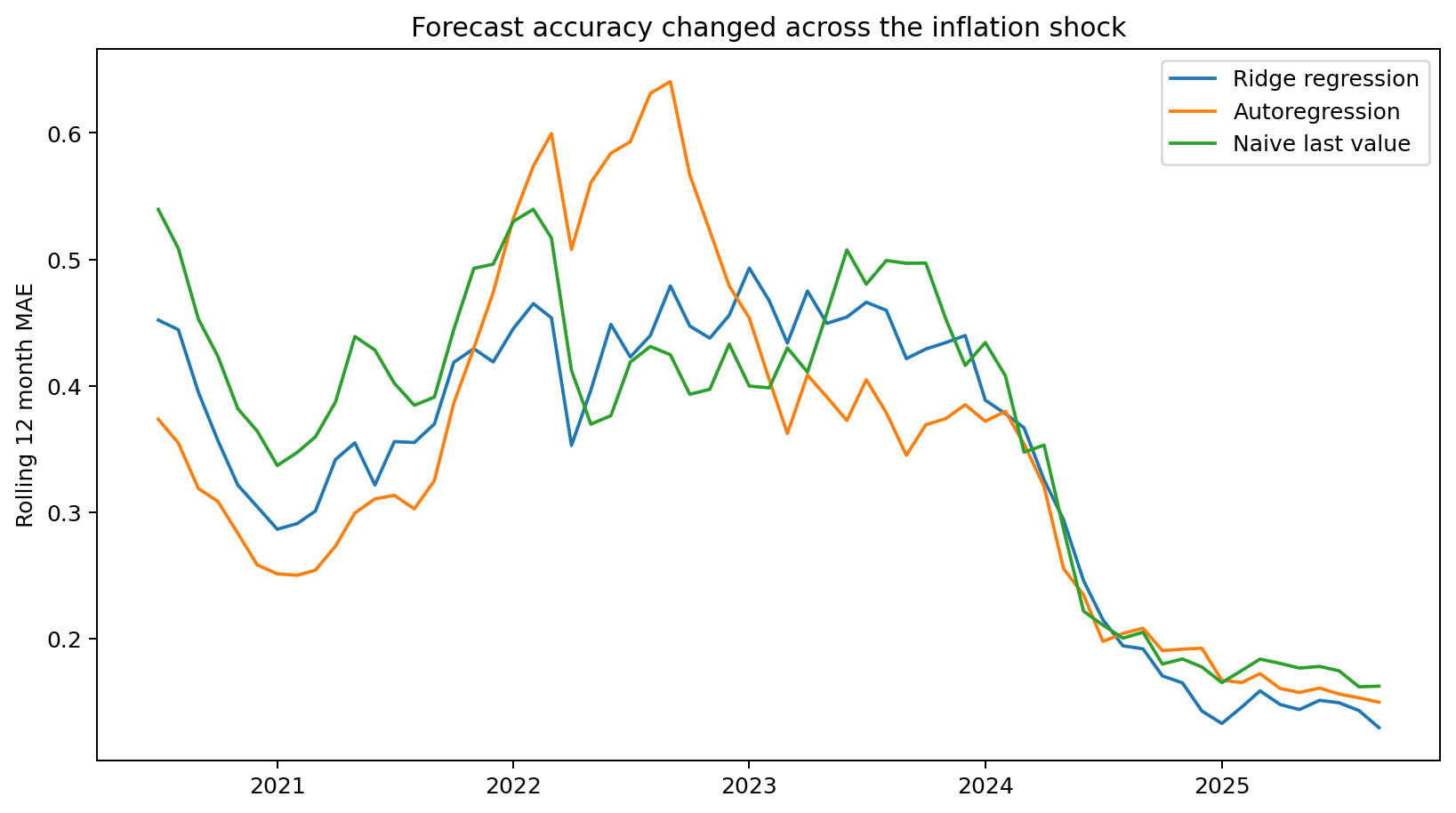
The rolling error chart also shows that model ranking changed through time. A forecaster should not look only at the average score. Ask when the model failed, how large the miss was, and whether the failure happened in the exact period that mattered most.
What research says about simple versus complex models
The broader research is less dramatic than many machine learning headlines. Federal Reserve work on real time U.S. inflation forecasting found that simple models remain hard to beat. The same research found that forecast combinations can improve accuracy and reduce the damage from a bad individual forecast. Forecasting inflation components separately can also help in some settings.
A 2025 IMF study on GDP nowcasting compared traditional econometric models with machine learning methods. In four of six country applications, dynamic factor or bridge models beat the machine learning alternatives. Among the machine learning choices, simpler methods such as Lasso and Elastic Net often performed better than more complex models. The authors point to a basic reason: GDP samples are short by machine learning standards.
This does not mean complex models are useless. It means they need data that justify their flexibility. When a project adds genuinely new information, such as large panels, text, transactions, or other timely signals, machine learning can create value that a small linear model cannot reach.
Model families: when each one makes sense
A useful model choice starts with the data, not the latest algorithm. The table below gives a practical first pass.
| Model family | Try it first when | Main strength | Main risk |
|---|---|---|---|
| Naive persistence | The series is persistent and the horizon is short | Hard baseline to beat | Misses turning points |
| Autoregression | Past values carry most of the signal | Simple and stable | Limited outside information |
| Ridge | Many predictors move together and sample is modest | Stable shrinkage and extrapolation | Still assumes mostly linear effects |
| Lasso or Elastic Net | You want shrinkage plus feature selection | Can simplify a wide feature set | Selected variables can change by sample |
| Random forest | There are nonlinear patterns and enough repeated examples | Captures interactions and thresholds | Weak extrapolation |
| Gradient boosting | Predictive patterns are nonlinear and tuning is careful | Often strong on structured data | Can overfit and fail outside training range |
| Neural network | You have a large data set or rich high frequency inputs | Flexible representation | Data hungry and harder to audit |
| Ensemble | Several models have different error patterns | Can improve stability | More moving parts to maintain |
GDP forecasting: machine learning is often a nowcasting problem
GDP arrives after much of the quarter has already happened. That makes current quarter nowcasting a natural use case for timely monthly data. Retail sales, industrial production, housing, trade, employment, and surveys can fill gaps before BEA publishes GDP.
The Atlanta Fed GDPNow system is a good reminder that strong production forecasting is often hybrid. It uses a dynamic factor model to fill missing monthly source data, then bridge equations and Bayesian vector autoregressions to estimate GDP components. It is not simply one black box model.
The St. Louis Fed Economic News Index is another example. It uses information from key monthly releases to update a real GDP nowcast through the quarter. As of August 21, 2026, its third quarter nowcast was about 1.93 percent at an annual rate.
For a machine learning GDP project, compare against bridge and factor models. If a complex model cannot beat those baselines across multiple quarters, it has not earned the extra complexity.
Inflation forecasting: persistence makes the baseline strong
Inflation is persistent, so the last value is a difficult short horizon benchmark. Useful features include core inflation, shelter, energy, food, wage growth, import prices, inflation expectations, and policy rates. But more features do not automatically improve the forecast.
Regularized linear models are often a good first machine learning choice because inflation predictors are correlated. Component models can also help. A model can forecast shelter, energy, and other parts separately, then combine them. Federal Reserve research has found value in component aggregation and forecast combinations in real time tests.
The biggest test is a regime change. If inflation moves outside the training range, ask whether the model can extrapolate or whether it simply repeats patterns it already saw.
Unemployment forecasting: watch the leading labor signals
The unemployment rate moves more slowly than many labor indicators. Initial claims, payroll growth, hours, vacancies, participation, temporary help employment, and financial conditions can provide earlier signals.
A linear model may work well during normal periods. Nonlinear models can become useful near sharp labor market breaks because relationships may change when layoffs spread. But the same flexibility can overfit a small number of downturns.
For unemployment, score both average error and turning point behavior. A model that is slightly better in calm months but misses every sharp rise may not be the model you want.
Recession prediction: the rare event problem
Recession prediction is a classification task when the target is recession or no recession. The main problem is not only model choice. It is the small number of recession episodes.
A model can achieve high accuracy by predicting expansion almost all the time. That is why probability calibration, precision, recall, Brier score, and false alarm rates matter. Time ordered validation is essential. The yield curve, labor data, financial conditions, credit, production, and income can all help, but no single signal is enough.
This is also where the related article U.S. Recession Indicators: A Data Driven Dashboard fits naturally. A dashboard can show the live signals, while a forecasting model can estimate a probability. They answer different questions and should remain separate pages.
Nowcasting versus forecasting
Nowcasting asks, what is happening now before the official data arrive? Forecasting asks, what happens later? Machine learning often looks stronger in nowcasting because the model can use fresh information that is closely tied to the current target.
Longer horizon forecasting is harder. The economy has more time to change, policy can react, and new shocks can appear. A model that wins one quarter ahead may fail four quarters ahead. Always report results by horizon.
How to evaluate a model fairly
Mean absolute error, or MAE, is easy to explain. It tells you the average size of the miss. Root mean squared error, or RMSE, gives more weight to large misses. Use both when large mistakes matter.
Directional accuracy can help when the question is whether growth rises or falls, but it should not replace size based errors. For recession probabilities, use calibration and probability scores rather than a single accuracy number.
A good results section should also report improvement versus the baseline, rolling error, the worst periods, and stability across horizons. A model that wins by 1 percent but fails badly during every recession may be less useful than a model with slightly higher average error and better stress performance.
- MAE for an easy average error measure.
- RMSE to expose large misses.
- Baseline improvement in percent.
- Rolling error to show changing performance.
- Worst period analysis to reveal structural breaks.
- Calibration for probability forecasts.
- Multiple horizons when the use case requires them.
Real time data and vintage data are not optional details
A revised data backtest answers a different question from a real time forecast test. If GDP was first reported at one value and later revised, a model trained on the revised history has information the real forecaster never had.
FRED and ALFRED provide real time periods and vintage date tools. For serious research, save the vintage used for every forecast. If that is not possible, label the analysis as a revised data exercise. Clear disclosure is better than false precision.
Release timing matters too. If the unemployment report was published on Friday, a forecast dated Thursday cannot use it. The same rule applies to CPI, GDP, retail sales, and every other feature.
Interpretability: useful, but not causality
Ridge coefficients can show the direction and size of a standardized relationship. Tree models can provide feature importance. Permutation importance asks how much performance falls when a feature is disturbed. SHAP values can explain how features contributed to a specific prediction.
These tools help explain the model. They do not prove that a variable caused the outcome. A strong feature may be a proxy for another part of the economy. Economic reasoning and causal research are separate tasks.
A production workflow that survives contact with new data
A forecasting model becomes useful when it can be rerun without changing the rules after every bad forecast. A simple production workflow is enough for many teams.
- Store raw data with source, series ID, release date, and vintage.
- Build features with code, not manual spreadsheet edits.
- Save the model version and training end date.
- Write the forecast to an archive before the target is released.
- Score the forecast automatically when the official value arrives.
- Track rolling MAE and RMSE.
- Set a rule for retraining and do not retrain only after a bad month.
- Review feature drift and missing releases.
- Keep a simple baseline live beside the main model.
Decision framework: which model should you try first?
There is no universal winner. The table below is a practical starting point, not a fixed rule.
| Data situation | Best first model to try | Why |
|---|---|---|
| Small monthly sample, many correlated predictors | Ridge or Elastic Net | Stable, simple, and hard to overfit compared with flexible trees |
| Quarterly GDP with timely monthly releases | Bridge or factor baseline, then regularized model | Traditional nowcasting methods are strong benchmarks |
| Clear nonlinear thresholds with enough history | Random forest or boosting | Can capture interactions that linear models miss |
| Many models are close but fail in different months | Simple ensemble | Averages model specific mistakes |
| Very large high frequency or text data | Regularized model first, then neural or boosting models | Complexity may be justified by the richer information set |
| Rare recession events | Probit or logistic baseline plus carefully validated machine learning | Few positive cases make flexible models easy to overfit |
| Need a transparent policy or business forecast | Ridge, Elastic Net, or simple ensemble | Easier to explain, monitor, and audit |
Limitations
The inflation comparison in this guide is one experiment. It uses one month ahead CPI, a specific feature set, and revised historical data. A true vintage test could produce different rankings.
Research findings also depend on country, target, horizon, and sample. A model that works for inflation may not work for GDP. A model that works in an expansion may fail during a crisis. The purpose of this guide is to show a testing framework, not to crown one algorithm.
Conclusion
Machine learning for economic forecasting works best when it is treated as a disciplined forecast comparison, not a contest for the most complex model.
For many U.S. macro problems, start with a naive or traditional baseline. Try Ridge or Elastic Net next when the sample is modest and predictors overlap. Add tree models when there is enough evidence for nonlinear patterns. Use ensembles when models fail in different periods. Use neural networks only when the data volume and use case justify them.
Most of all, protect the test. Use time ordered validation, real time data when possible, clear forecast horizons, and a live baseline. If a complex model loses, keep the loss. That result is often more useful than a polished win.
Method note and reproducibility
The inflation benchmark summarized in this pillar guide comes from the companion article Inflation Forecasting With Machine Learning: A Reproducible Test. The final holdout covers target months from February 2020 through September 2025. Ridge used alpha 10. Random forest used 600 trees, maximum depth 6, and minimum leaf size 6. Gradient boosting used 400 estimators, depth 2, and learning rate 0.03. Tree model random seed was 42.
The test used official BLS CPI series for the target and CPI components, with FRED used for macro context and series definitions. It is a revised data exercise, not a full ALFRED vintage backtest. The ranking is evidence from one design, not a universal result.
Primary sources
- Google Search Central, Creating helpful, reliable, people first content
- Google Search Central, Article structured data
- Google Search Central, Canonicalization
- FRED API, series observations and vintage dates
- BLS, Consumer Price Index, July 2026
- FRED, Unemployment Rate, UNRATE
- BEA, GDP second estimate, second quarter 2026
- FRED, St. Louis Fed Economic News Index real GDP nowcast
- Atlanta Fed, GDPNow current and past commentaries
- Federal Reserve, Machine Learning, the Treasury Yield Curve and Recession Forecasting
- Federal Reserve, Forecasting US inflation in real time
- IMF, GDP Nowcasting Performance of Traditional Econometric Models vs Machine Learning Algorithms
Financial information note
This article is for research and education. Forecasts are estimates, not guarantees. Do not use one model output alone for investment, borrowing, pricing, hiring, or policy decisions.
Downloads
Files attached to this article for your reference.