
Mean and Median: A Student-Friendly Guide to Measures of Central Tendency
A student-friendly guide to measures of central tendency, with ungrouped and grouped-data methods, formulas, calculations, strengths, and limitations.
Mean and Median
A student-friendly guide to measures of central tendency, with ungrouped and grouped-data methods, formulas, calculations, strengths, and limitations.
In statistics, a measure of central tendency is a single value used to represent the centre or typical level of a set of observations. Two of the most important measures are the arithmetic mean and the median. They both describe the “middle” of data, but they do so in different ways.
1. Why do we need a measure of central tendency?
A raw list of observations can be difficult to interpret, especially when the data set is large. A measure of central tendency condenses the data into one representative value. The source text explains that a satisfactory average should be clearly defined, based on the observations, simple to understand, easy to calculate, suitable for mathematical treatment, relatively stable from sample to sample, and not unduly influenced by unusually large or small observations.
2. Arithmetic Mean
The arithmetic mean, usually called the mean, is found by adding all observations and dividing the total by the number of observations. It is the most familiar numerical average.
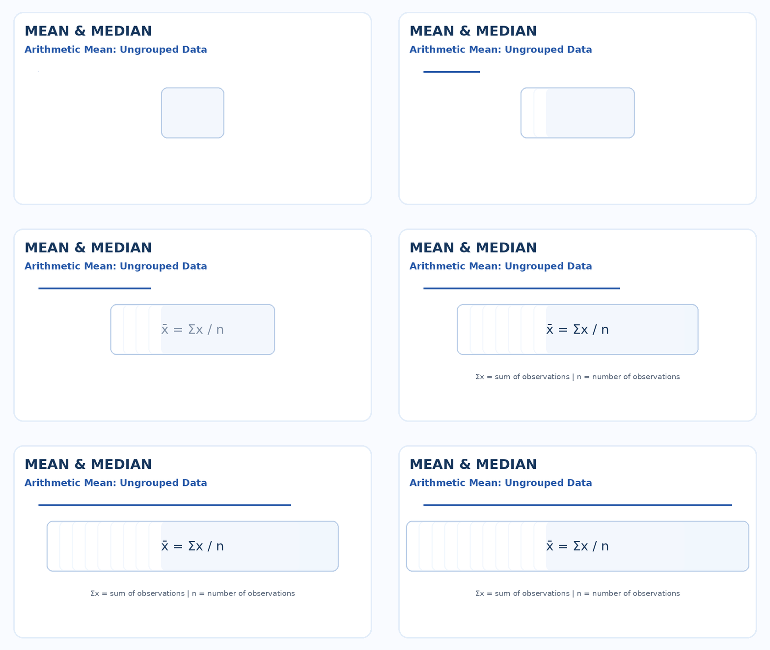
Here, ( bar{x} ) is the sample mean, ( ∑ x ) means “add all the observations,” and ( n ) is the number of observations.
2.1 Mean for ungrouped data: Direct method
Ungrouped data are individual values listed separately. For this type of data, the direct method is the simplest approach.
- Add all the observations.
- Count how many observations there are.
- Divide the total by the number of observations.
Example. Find the mean of the following marks:
45, 32, 37, 46, 39, 36, 41, 48, 36
( bar{x} = {360}/{9} = 40 )
Therefore, the mean mark is 40.
2.2 Mean for grouped data: Midpoint-frequency method
When there are many observations, data are often arranged into class intervals with frequencies. In grouped data we usually do not know every original observation, so each class is represented by its midpoint.
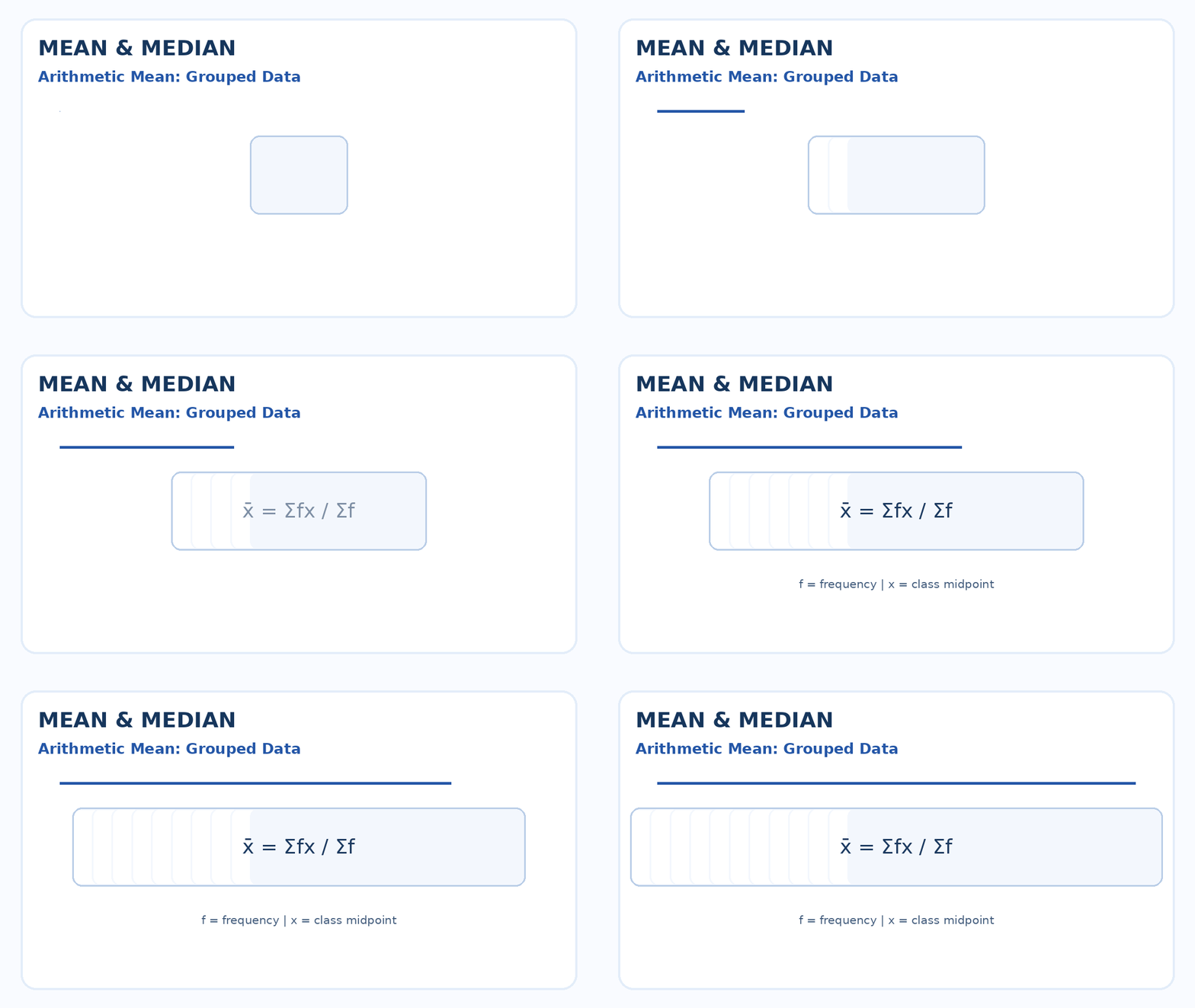
In this formula, ( f ) is the frequency of a class and ( x ) is the midpoint of that class. The midpoint is found by:
Class midpoint = (Lower class limit + Upper class limit) ÷ 2
Example. The grouped weights below are adapted from the source example.
| Weight (g) | Frequency, f | Midpoint, x | fx |
|---|---|---|---|
| 65–84 | 9 | 74.5 | 670.5 |
| 85–104 | 10 | 94.5 | 945.0 |
| 105–124 | 17 | 114.5 | 1946.5 |
| 125–144 | 10 | 134.5 | 1345.0 |
| 145–164 | 5 | 154.5 | 772.5 |
| 165–184 | 4 | 174.5 | 698.0 |
| 185–204 | 5 | 194.5 | 972.5 |
| Total | 60 | 7350.0 |
Therefore, the approximate mean weight from the grouped distribution is 122.5 g.
2.3 A second grouped-data example for the mean
The same midpoint-frequency method can be taught with a smaller table so that students can see every step clearly. Suppose the marks of 20 students are grouped as follows:
| Marks | Frequency, f | Midpoint, x | fx |
|---|---|---|---|
| 0–10 | 2 | 5 | 10 |
| 10–20 | 5 | 15 | 75 |
| 20–30 | 7 | 25 | 175 |
| 30–40 | 4 | 35 | 140 |
| 40–50 | 2 | 45 | 90 |
| Total | 20 | 490 |
Step 1: Find the midpoint of each class.
Step 2: Multiply each midpoint by its class frequency to obtain (fx).
Step 3: Add the frequencies and the (fx) values.
( ∑ f = 20 ) and ( ∑ fx = 490 )
Step 4: Apply the grouped-mean formula.
Therefore, the estimated mean mark is 24.5.
2.4 Strengths and limitations of the mean
Strengths
- It is precisely and mathematically defined.
- It uses all observations in the data set.
- It is easy to calculate and easy to understand.
- It is relatively stable from sample to sample.
- It is suitable for further algebraic and statistical treatment.
Limitations
- It is strongly affected by extremely large or extremely small values.
- It can sometimes give a value that is not typical of any actual observation.
- In highly skewed distributions, it may not represent the centre well.
- With open-ended classes, it cannot usually be calculated without making assumptions about the missing class limits.
Illustration of sensitivity to extremes: Compare the values 10, 11, 12, 13, 14 with 10, 11, 12, 13, 100. The extreme value 100 pulls the mean sharply upward. This is an important reason to consider the median when data are skewed.
3. Median
The median is the value that divides an ordered data set into two equal parts. About half of the observations lie below it and half lie above it. Unlike the mean, the median is an average of position.
3.1 Median for ungrouped data: Ordered-position method
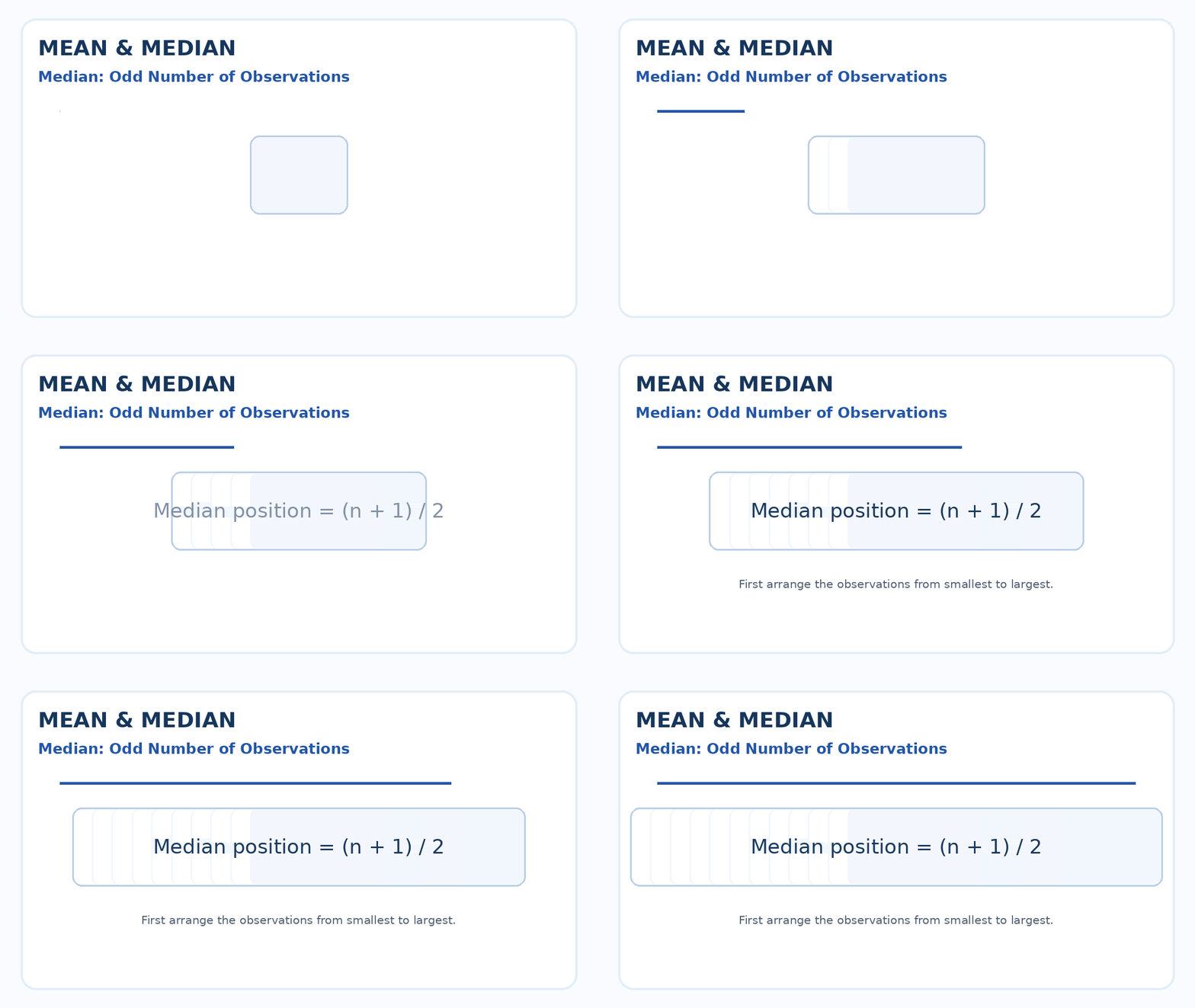
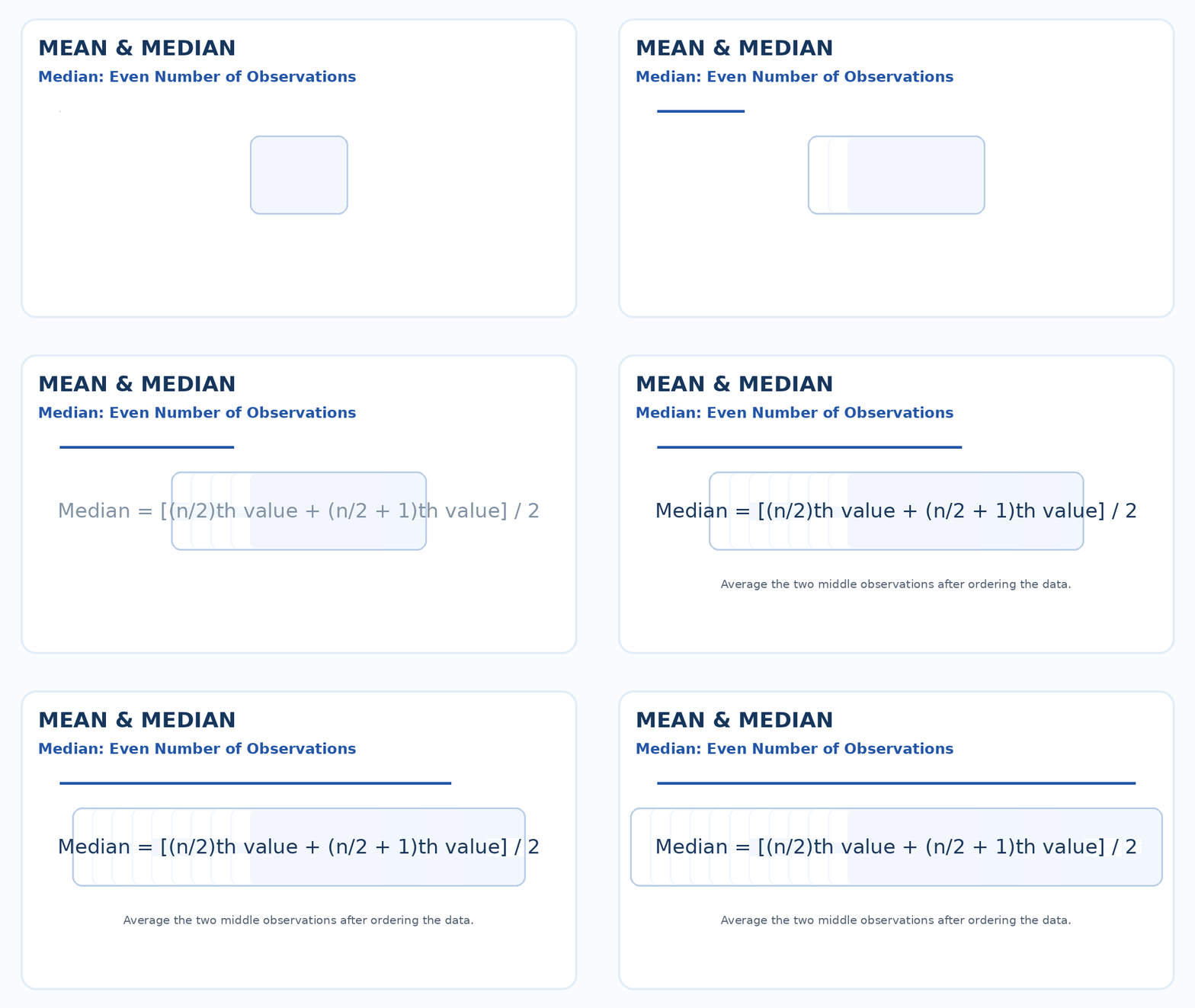
For ( n ) observations arranged in ascending order:
Example. Find the median of:
45, 32, 37, 46, 39, 36, 41, 48, 36
First arrange the observations:
32, 36, 36, 37, 39, 41, 45, 46, 48
There are ( n = 9 ) observations, so the median position is:
The 5th observation is 39.
Therefore, the median is 39 marks.
3.2 Median for grouped data: Linear interpolation method
In continuous grouped data, the exact middle observation may lie somewhere inside a class interval. The source calculates the median by linear interpolation inside the median class.
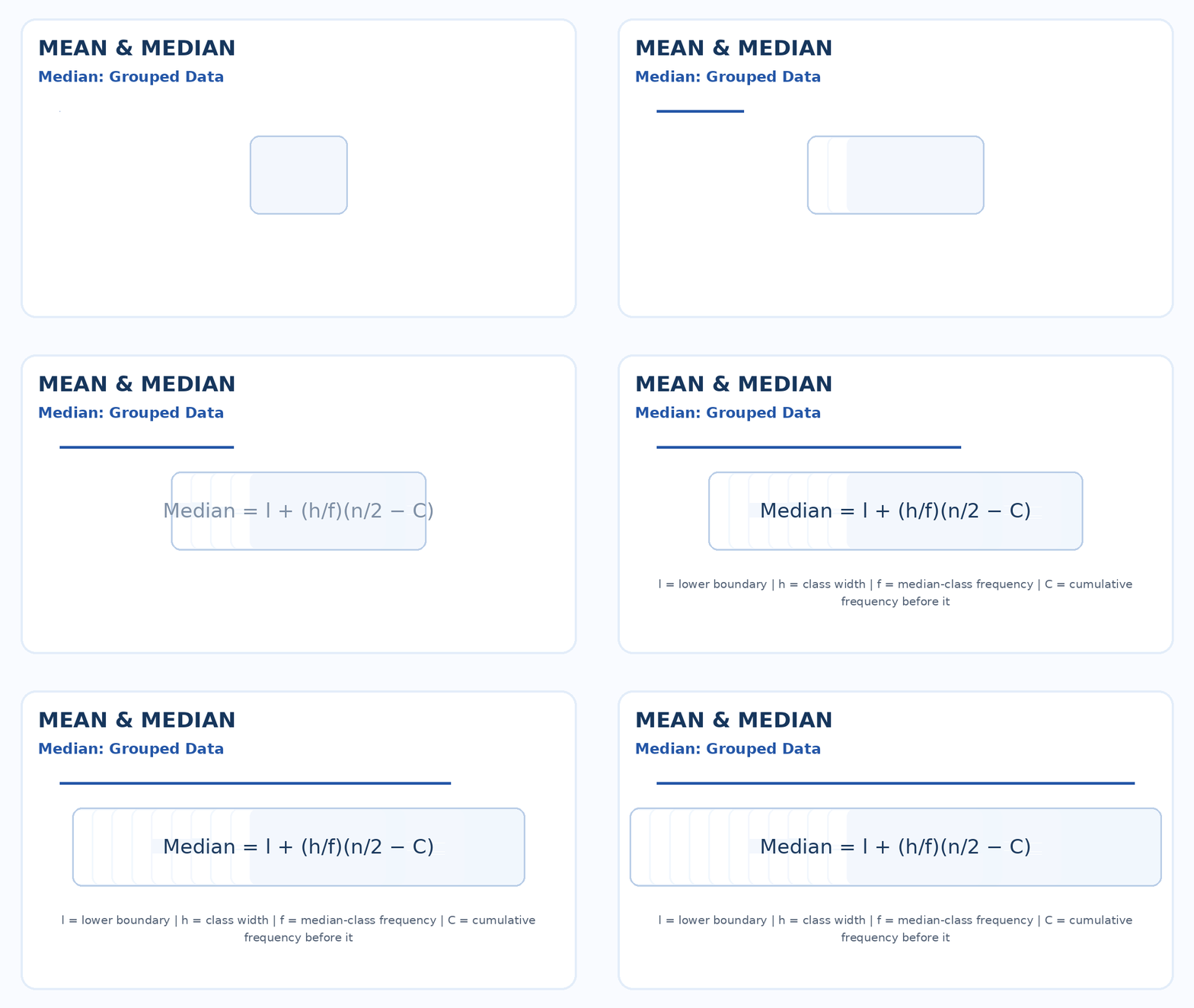
where:
- ( L) = lower class boundary of the median class
- ( h ) = class width
- ( f ) = frequency of the median class
- ( n ) = total frequency
- ( c ) = cumulative frequency before the median class
Example. Consider the grouped examination marks below.
| Class boundaries | Frequency | Cumulative frequency |
|---|---|---|
| 29.5–39.5 | 8 | 8 |
| 39.5–49.5 | 87 | 95 |
| 49.5–59.5 | 190 | 285 |
| 59.5–69.5 | 304 | 589 |
| 69.5–79.5 | 211 | 800 |
| 79.5–89.5 | 85 | 885 |
| 89.5–99.5 | 20 | 905 |
Total frequency ( n = 905). The median position is:
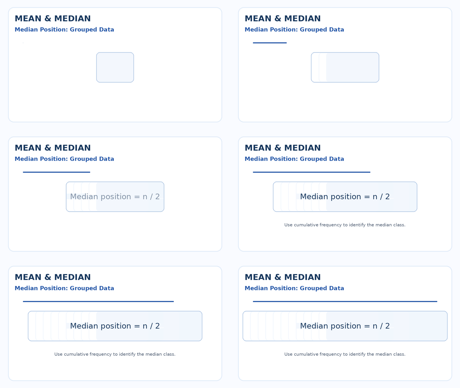
The 452.5th observation lies in the class 59.5–69.5 because the cumulative frequency rises from 285 to 589 in that class. Therefore:
( l = 59.5; h = 10; f = 304; C = 285)
( approx 59.5 + 5.5 = 65)
Therefore, the grouped median is approximately 65 marks.
3.3 A second grouped-data example for the median
For grouped data, the median is found by first identifying the class that contains the middle observation. Consider the following distribution of marks:
| Marks | Frequency, f | Cumulative frequency |
|---|---|---|
| 0–10 | 3 | 3 |
| 10–20 | 5 | 8 |
| 20–30 | 9 | 17 |
| 30–40 | 7 | 24 |
| 40–50 | 6 | 30 |
| Total | 30 |
Step 1: Find the middle position.
The 15th observation lies in the class 20–30 because the cumulative frequency is 8 before this class and rises to 17 in this class. Therefore, 20–30 is the median class.
Step 2: Identify the quantities needed in the formula.
Step 3: Substitute into the grouped-median formula.
Therefore, the estimated median mark is approximately 27.78.
3.4 Strengths and limitations of the median
Strengths
- It is easy to understand and usually easy to calculate.
- It is not greatly affected by extremely large or small values.
- It can be used for open-ended distributions.
- It is especially useful for skewed distributions, such as income, house prices, and similar data.
Limitations
- It is not as rigidly defined algebraically as the arithmetic mean.
- It does not use the numerical size of every observation.
- It is not well suited to further algebraic manipulation.
- For a large ungrouped data set, arranging all observations in order can be time-consuming.
4. Mean versus Median: Which should students use?
| Question | Mean | Median |
|---|---|---|
| Uses every observation? | Yes | No, mainly depends on order and position |
| Affected by extreme values? | Strongly | Much less |
| Useful for skewed data? | Sometimes misleading | Often preferred |
| Suitable for algebraic/statistical treatment? | Very suitable | Limited |
| Can work with open-ended classes? | Usually difficult | Often possible |
| Main interpretation | Balance point / arithmetic average | Middle position |
5. Common student mistakes
- Forgetting to order data before finding the median.
- Using class limits instead of class midpoints when calculating a grouped mean.
- Choosing the grouped median class incorrectly. First locate ( n/2 ) in the cumulative-frequency column.
- Confusing frequency with cumulative frequency. Frequency is the number in one class; cumulative frequency is the running total.
- Treating a grouped mean as exact. It is usually an approximation because midpoints represent whole classes.
6. Quick practice
Practice A, ungrouped mean: Find the mean of 8, 10, 12, 15, 20.
Answer: ( (8+10+12+15+20)/5 = 13).
Practice B, ungrouped median: Find the median of 5, 9, 11, 13, 18, 25.
Answer: ( (11+13)/2 = 12).
7. Summary
The mean and median are both measures of central tendency, but they answer slightly different questions. The mean asks, “What is the arithmetic average of all values?” The median asks, “What value lies in the middle after the observations are ordered?” For ungrouped data, both can be calculated directly from individual observations. For grouped data, the mean is commonly estimated with class midpoints and frequencies, while the median is found by locating the median class and applying linear interpolation.
Understanding both measures is important because a single “average” can be misleading if students do not consider the shape of the distribution, extreme values, and the way the data have been grouped.