Odds Ratio Calculator and Interpretation

An odds ratio (OR) compares the odds of an outcome between two groups. An OR of 1 means equal odds, an OR above 1 means higher odds in the group of interest, and an OR below 1 means lower odds. This odds ratio calculator and interpretation guide helps you calculate the OR, 95% confidence interval and p-value, then decide what the result actually means.

The number alone is not enough. A defensible interpretation also checks the reference group, the confidence interval, the study design, baseline event rates, and whether the odds ratio is being mistaken for a risk ratio. Those checks matter because an OR can be mathematically correct yet still be communicated in a misleading way.

Odds Ratio Calculator: Calculate OR, 95% CI, and P-Value

Interactive calculator: Use the accompanying HTML file for live OR, 95% CI, Wald p-value, observed risks and RR. The calculation compares exposed/treatment with unexposed/control and automatically labels a 0.5 zero-cell correction when used.

	Outcome present	Outcome absent
Exposed / treatment	a = 30	b = 20
Unexposed / control	c = 10	d = 40

Example calculator result: OR = 6.000; 95% CI 2.453 to 14.678; Wald p < 0.0001; observed RR = 3.00.

What each input means

Cell	Meaning
a	Exposed or treatment participants with the outcome
b	Exposed or treatment participants without the outcome
c	Unexposed or control participants with the outcome
d	Unexposed or control participants without the outcome

Before interpreting the result, verify the direction of comparison. Reversing the groups or reversing event and non-event changes the OR to its reciprocal. An OR of 4.0 becomes 0.25 when the comparison is reversed. Cochrane uses the same reciprocal relationship to explain why ratio measures are naturally analysed on a logarithmic scale.

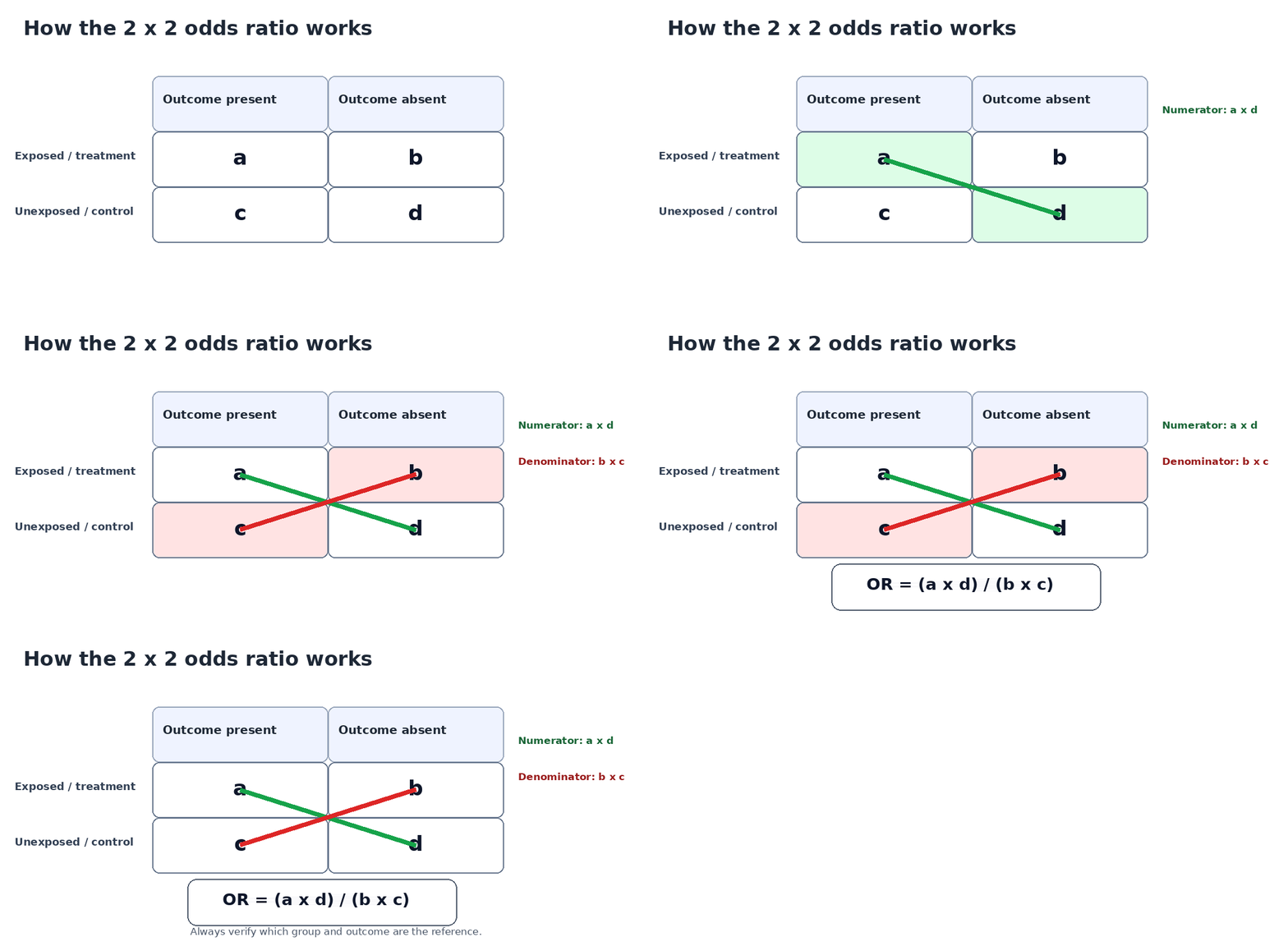
Animation: the cross-product calculation OR = (a x d) / (b x c).

What happens if one cell contains zero?

A zero cell can make the ordinary sample OR equal to zero or infinity and can make the log standard error undefined. A common continuity correction is to add 0.5 to all four cells. Cochrane describes this as a customary approach when zero cells prevent conventional calculation, and MedCalc uses the same correction in its calculator.

The correction is a computational device, not additional observed data. If event counts are sparse, the point estimate can remain unstable and the interval can remain very wide. In that setting, the main lesson is not to “fix” the table until the result looks clean, but to use a method appropriate to the data and report the uncertainty honestly.

Important limitation: A simple 2 x 2 calculator is designed for an appropriate table of independent observations. Matched case-control data, repeated observations, clustered data and other dependent designs can require different methods because naive standard errors may be wrong. [1]

What Is an Odds Ratio in Simple Terms?

An odds ratio answers a specific question: how do the odds of an outcome in one group compare with the odds in another group? It is a measure of association for a binary outcome such as disease/no disease, success/failure or event/no event.

Odds vs probability: the distinction that prevents most errors

If 20 of 100 people experience an outcome, the probability is 20/100 = 0.20, or 20%. The odds are 20/80 = 0.25 because odds compare events with non-events. More generally, if the probability is p, the odds are p/(1-p).

Risk and odds are close when an event is uncommon, but they separate as the event becomes common. Cochrane illustrates that a risk of 0.50 corresponds to odds of 1, while a risk of 0.95 corresponds to odds of 19.

Why odds and risk are not interchangeable

Suppose the odds of an outcome are 0.50 in the exposed group and 0.25 in the unexposed group. The OR is 2.0, so the exposed group has twice the odds. That does not automatically mean twice the probability or twice the risk.

This wording is more than statistical etiquette. When an outcome is common, describing an OR as though it were a risk ratio can make the effect sound much larger than the underlying difference in probability. Altman, Deeks and Sackett highlighted this communication problem in BMJ, and Cochrane continues to warn that OR and RR are different valid measures that should not be confused.

How Is the Odds Ratio Calculated?

For the standard 2 x 2 table, the odds ratio is the cross-product ratio:

OR = (a x d) / (b x c)

The same formula can be written as the odds in the exposed group divided by the odds in the unexposed group:

OR = (a / b) / (c / d)

The CDC presents the same 2 x 2 notation and cross-product calculation in its epidemiology training material.

Standard error of the log odds ratio

A commonly used large-sample standard error is calculated on the natural-log scale:

SE[ln(OR)] = sqrt(1/a + 1/b + 1/c + 1/d)

Ratio measures such as OR are analysed on the log scale because the original scale runs from 0 to infinity with 1 as the null value. The log transformation makes reciprocal effects symmetric around zero.

How the 95% confidence interval is calculated

The common log-Wald interval is:

95% CI = exp[ ln(OR) +/- 1.96 x SE(ln OR) ]

This is the method used by the calculator on this page. It works well as a conventional large-sample approximation but can perform poorly with very sparse data or extreme cell counts. MedCalc documents the same OR, standard-error and log-Wald formulas.

How the p-value is calculated here

The calculator uses the corresponding Wald statistic z = ln(OR) / SE[ln(OR)] and a two-sided normal-theory p-value. This keeps the displayed p-value aligned with the displayed Wald confidence interval in ordinary large-sample use.

Other tools may use Fisher's exact test, a chi-square test, an exact confidence interval or a model-based interval. Those procedures are not automatically interchangeable in small discrete tables. Michael Fay showed that a two-sided Fisher exact test and the usual exact OR confidence interval can occasionally lead to apparently conflicting inferences because the test and interval are not exact inverses of the same two-sided procedure.

How to Interpret an Odds Ratio

The cleanest interpretation has five parts: direction, magnitude, precision, statistical evidence and practical relevance. Reading only whether OR is above or below 1 leaves out most of what matters.

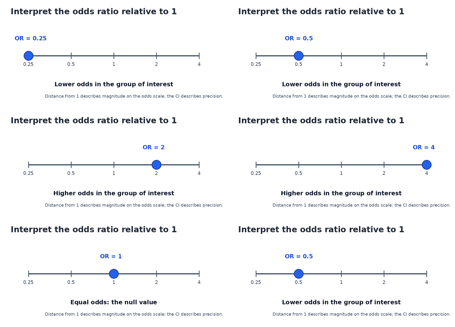
Animation: OR is interpreted relative to the null value of 1.

OR = 1: equal odds

An OR of exactly 1 means the observed odds are equal in the two groups. It is the null value for the odds-ratio scale.

OR > 1: higher odds

If OR = 2.5, the group in the numerator has 2.5 times the odds of the outcome relative to the reference group. You can also say the odds are 150% higher because (2.5 - 1) x 100 = 150%.

Do not silently replace “odds” with “risk.” OR = 2.5 does not generally mean a 150% increase in risk.

OR < 1: lower odds or an inverse association

If OR = 0.40, the group in the numerator has 0.40 times the odds, or 60% lower odds, because (1 - 0.40) x 100 = 60%.

In observational research, “lower odds” or “inverse association” is usually safer than automatically calling the exposure “protective.” An OR describes association; causal language requires a design and analysis that justify causal interpretation.

Does a larger OR always mean a stronger or more important effect?

Farther from 1 means a larger relative difference on the odds scale, but it does not automatically mean more important. An OR of 8 with a 95% CI of 0.8 to 80 is highly uncertain. An OR of 1.8 with a narrow interval may be more informative about the likely size and direction of the association.

Practical importance also depends on baseline probability, severity of the outcome, absolute differences, costs, harms and study quality. Statistical magnitude and decision importance are related, but they are not the same question.

How to Interpret the 95% Confidence Interval

The confidence interval adds the information that the point estimate cannot: precision. A narrow interval gives a more precise estimate than a wide interval, assuming the model and study assumptions are reasonable.

What it means when the 95% CI includes 1

If the interval is 0.75 to 2.10, it includes the null value of 1. Under the corresponding conventional two-sided 5% procedure, the data do not provide enough evidence to reject the null.

That is not the same as proving “no association.” The data may simply be compatible with a broad range of effects because the study is imprecise.

What it means when the 95% CI excludes 1

If the interval is 1.45 to 3.12, it lies entirely above 1. With the corresponding two-sided procedure, that is statistical evidence against the null at approximately the 5% level. The same logic applies to an interval entirely below 1.

Why the word “corresponding” matters

A 95% CI that excludes 1 and a p-value below 0.05 line up cleanly when the interval and test are based on corresponding methods. Sparse-data tools sometimes mix a Wald interval with Fisher's exact p-value or pair a two-sided exact test with a nonmatching exact interval. If the results appear inconsistent, first check the method labels rather than assuming one calculator is wrong.

Odds Ratio Examples With Step-by-Step Interpretation

Example: higher odds, but OR and RR are not the same

Group	Outcome present	Outcome absent
Exposed	30	20
Unexposed	10	40

The odds ratio is (30 x 40)/(20 x 10) = 6.00. Using the log-Wald method, the approximate 95% CI is 2.45 to 14.68.

The exposed group therefore has six times the odds of the outcome. But the observed risks are 30/50 = 60% and 10/50 = 20%, so the risk ratio is only 3.0. Both numbers are correct because they describe different scales.

Example: lower odds

Group	Outcome present	Outcome absent
Exposed	10	40
Unexposed	25	25

The OR is 0.25 with an approximate 95% CI of 0.10 to 0.61. The exposed group has 75% lower odds of the outcome.

The observed risks are 20% and 50%, giving RR = 0.40, or a 60% lower risk. Again, the percentage reduction in odds is not the same as the percentage reduction in risk.

Example: OR close to 1 with little precision

If the exposed group has 22 events and 78 non-events while the control group has 20 events and 80 non-events, OR is approximately 1.13 and the log-Wald 95% CI is approximately 0.57 to 2.23. The estimate is close to the null and the interval remains compatible with both lower and higher odds.

Example: the point estimate is above 1 but the CI crosses 1

With 16 events and 34 non-events in the exposed group versus 10 events and 40 non-events in the comparison group, OR is approximately 1.88 and the 95% CI is approximately 0.76 to 4.69. The point estimate suggests higher odds, but the data are too imprecise to establish a clear direction under the conventional Wald framework.

Odds Ratio vs Relative Risk: What Is the Difference?

Relative risk (RR), also called the risk ratio, compares probabilities directly. OR compares odds. Cochrane treats OR, RR and risk difference as distinct effect measures for binary outcomes; none should be substituted for another without changing the interpretation.

RR = [a / (a+b)] / [c / (c+d)]

Why OR and RR diverge as baseline risk rises

For a fixed OR, the corresponding risk ratio depends on the baseline event probability. If the baseline risk is p0, the risk in the comparison group implied by a given OR can be written as p1 = OR x p0 / (1 - p0 + OR x p0).

For example, with OR = 3, a 1% baseline risk corresponds to a compared risk of about 2.9% and RR about 2.94. At a 20% baseline risk, the same OR corresponds to a compared risk of about 42.9% and RR about 2.14. At a 50% baseline risk, the compared risk is 75% and RR is only 1.50.

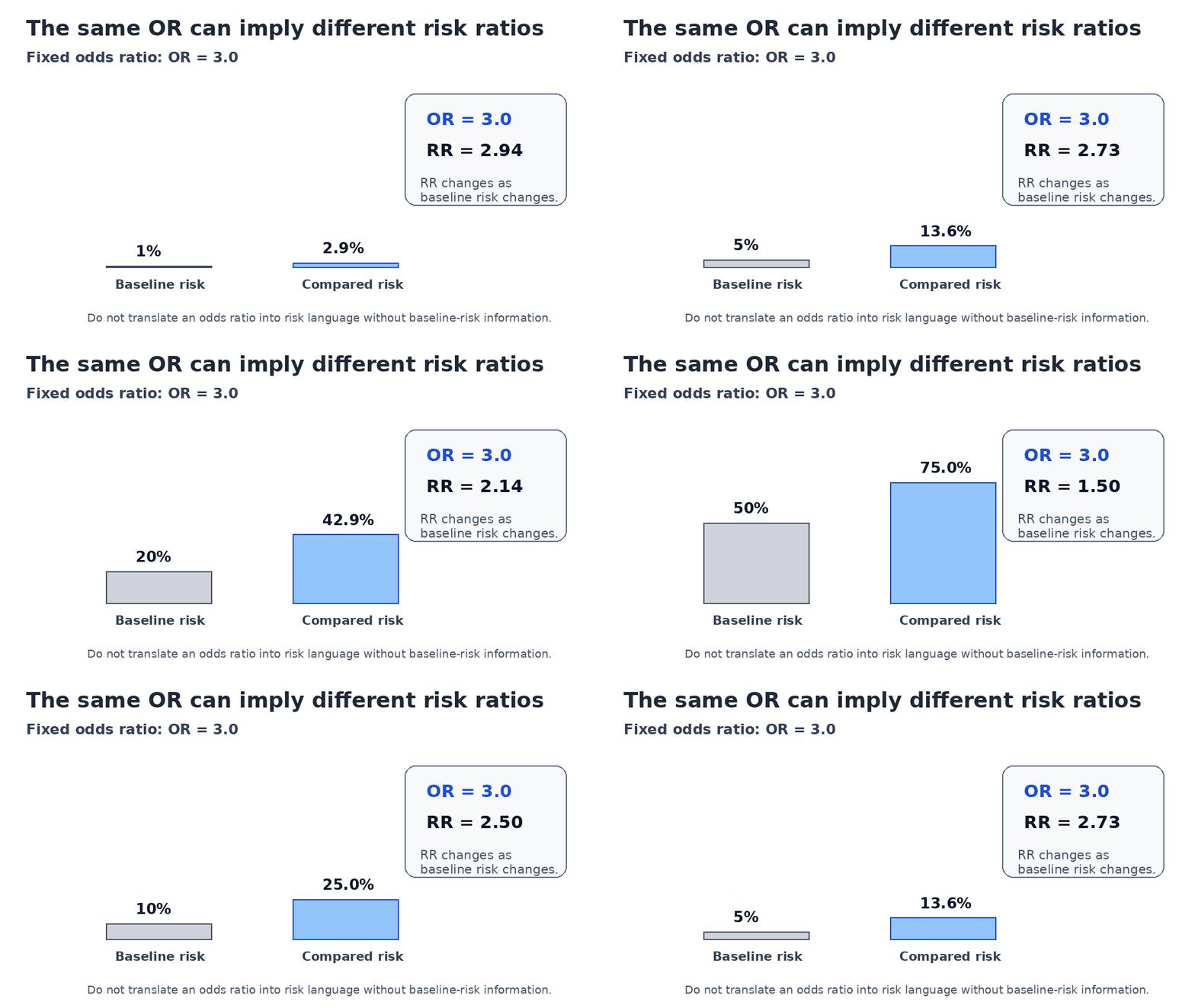
Animation: a fixed OR does not imply a fixed RR. Baseline risk changes the risk interpretation.

When does OR approximate RR?

OR and RR become numerically closer as the outcome becomes uncommon. There is no universal threshold at which they suddenly become equivalent. Rules such as “below 10%” are useful heuristics in some contexts, not a mathematical switch.

The CDC illustrates the approximation with uncommon outcomes, while Greenland and Thomas showed an important case-control nuance: when incidence-density sampling is used, an OR can estimate an incidence-rate ratio without requiring a rare-disease assumption. Rarity is especially relevant when an OR is being used as an approximation to a risk ratio.

Should you report OR or RR?

Situation	Usually most useful interpretation
Typical case-control study	OR is central; interpretation depends on the control-sampling design.
Cohort study	RR and absolute risk difference are directly available and often easier to communicate; OR may still be used for specific models.
Randomized trial	Report observed event rates and consider RR and absolute effects; OR may be appropriate for a prespecified logistic model.
Cross-sectional study	OR is a prevalence odds ratio; prevalence ratio may be easier to interpret when the outcome is common.
Logistic regression	Exponentiated coefficients naturally produce ORs; distinguish adjusted from crude effects.

The practical principle is simple: use OR when the design or model naturally estimates odds, but do not hide directly observable risks when they are available and useful for decisions.

When Should You Use an Odds Ratio?

Case-control studies

In a typical case-control study, researchers sample cases and controls rather than observing population risks directly. That is why OR is a standard measure of association in this design. The CDC notes that risk ratios usually cannot be calculated directly from the sampled case-control table because the investigator determines the number of controls.

A deeper point is that the effect estimated by the case-control OR depends on how controls were sampled. Pearce described how density sampling, sampling from a cohort at risk, and survivor sampling correspond to different underlying effect interpretations.

Cohort, cross-sectional and clinical studies

These designs can still use OR, but OR is not automatically the clearest effect measure. When actual risks or prevalences are observable, RR, prevalence ratio and absolute differences can be easier for clinicians, patients and policy readers to interpret.

When the outcome is common, the important problem is not that OR becomes invalid. It remains a valid odds-based measure. The problem is that translating it into risk language becomes increasingly misleading.

Logistic regression

Logistic regression models the log odds of a binary outcome. If a regression coefficient is beta, exponentiating it gives the odds ratio:

OR = exp(beta)

UCLA OARC demonstrates this directly: the coefficient is a change in log odds, and its exponential is the multiplicative change in odds. Statistical packages may display the result as an odds ratio or, in SPSS, as Exp(B).

Crude vs Adjusted Odds Ratios

A crude OR comes directly from the 2 x 2 table. An adjusted OR usually comes from a model such as multivariable logistic regression that includes other predictors or covariates.

If a model includes age, smoking status and disease severity, the adjusted OR for the exposure is interpreted conditional on the model specification and the included variables. A basic 2 x 2 calculator cannot reproduce that adjusted estimate from the four marginal counts alone.

Why the crude and adjusted OR can differ

Confounding is one possible reason, but it is not the only one. Odds ratios are non-collapsible: marginal and conditional ORs can differ even when there is no conventional confounding. Greenland discusses this property and why it should not be confused with confounding.

This is why “the adjusted OR changed, so confounding was present” is too simplistic. Interpretation should consider the causal question, model specification and the mathematical properties of the effect measure.

Common Odds Ratio Interpretation Mistakes and Troubleshooting

Mistake: saying OR = 2 means “twice as likely”

“Twice as likely” is usually understood as twice the probability. The safer wording is “twice the odds.” If the audience needs risk, calculate or report risk directly when the study design permits it.

Mistake: ignoring which group is the reference

If one program reports OR = 0.25 and another reports OR = 4.0, both can be correct if the reference group was reversed. Check the coding before looking for a software error.

Problem: the confidence interval is extremely wide

Wide intervals commonly reflect small samples, sparse events, imbalanced cells or weak information. A large point estimate with a huge interval should be reported as uncertain, not simply described as a “strong association.”

Problem: another calculator gives a different p-value

First compare the methods. One calculator may use a Wald z-test, another Pearson chi-square and another Fisher's exact test. They can differ, particularly in small samples. Also check continuity corrections, rounding, reference coding and whether one result is adjusted while the other is crude.

Mistake: treating statistical significance as practical importance

A large study can make a small association statistically precise. A small study can produce a large-looking OR with poor precision. Decisions should consider effect magnitude, absolute risk, uncertainty and real-world consequences rather than using p < 0.05 as the sole criterion.

Mistake: assuming OR proves causation

An odds ratio measures association. Causal interpretation depends on design and assumptions, including randomization when applicable, confounding control, selection processes, measurement quality and temporal ordering.

How to Report an Odds Ratio in Research

A useful results statement identifies the comparison, the outcome, the OR, the confidence interval and whether the estimate is crude or adjusted. The methods section should state how the interval and p-value were obtained.

Example, crude result: “Participants in the exposed group had higher odds of the outcome than participants in the unexposed group (OR 2.40, 95% CI 1.35-4.27).”

Example, adjusted result: “After adjustment for the prespecified covariates, exposure was associated with higher odds of the outcome (aOR 2.10, 95% CI 1.25-3.53).”

Use “associated with” rather than “caused” unless the study design and causal analysis support causal language. If risks can validly be estimated, reporting event rates or an absolute effect alongside the OR often makes the result easier to understand.

What to include in tables and figures

Make the modeled outcome and reference category explicit. For regression models, identify whether estimates are crude or adjusted and describe the adjustment variables or model strategy. If a correction or nonstandard interval was used for sparse data, label it.

Limitations of Odds Ratios

Odds ratios are useful, but they do not answer every practical question. The most important limitations arise when readers want probabilities, absolute effects or causal conclusions from a statistic that only reports relative odds.

Limitation	Why it matters
Does not show absolute risk	OR = 3 can describe very different probability changes depending on baseline risk.
Can be misread as RR	The discrepancy can be large when events are common.
Sensitive to sparse information	Small or zero cells can produce extreme estimates and wide intervals.
Does not establish causality	Study design and bias control remain essential.
Non-collapsibility	Adjusted and marginal ORs can differ even without ordinary confounding.
Simple 2 x 2 methods assume suitable independence	Matched, clustered or repeated data may need specialized models.

Frequently Asked Questions About Odds Ratios

What is considered a good odds ratio?

There is no universal “good” OR. The importance of an OR depends on the outcome, baseline probability, precision, study design and practical consequences. OR = 1.5 can be important for a severe outcome and unimportant for a trivial one.

Is an odds ratio of 2 statistically significant?

Not necessarily. Statistical significance depends on uncertainty, not only the point estimate. OR = 2 with a 95% CI of 1.3-3.1 provides different evidence from OR = 2 with a CI of 0.6-6.5.

Can an odds ratio be negative?

No. An OR ranges from zero toward infinity. OR = 1 is the null value. Values below 1 indicate lower odds and values above 1 indicate higher odds.

Can an odds ratio be zero?

A sample OR can be zero when the numerator cross-product is zero while the denominator is positive. However, ln(0) is undefined, so ordinary log-based standard errors and confidence intervals fail. Sparse-data methods or continuity corrections may then be needed.

What does an odds ratio of 0.5 mean?

OR = 0.5 means the group of interest has half the odds of the outcome, or 50% lower odds, relative to the reference group. Reversing the comparison gives 1/0.5 = 2.

What does an odds ratio of 2 mean?

OR = 2 means the group of interest has twice the odds of the outcome relative to the reference group. It does not automatically mean twice the risk.

How do you interpret an OR of 3?

OR = 3 means three times the odds of the outcome. The corresponding change in probability depends on baseline risk, so risk language requires additional information.

How do you convert an odds ratio to a percentage?

For OR above 1, (OR - 1) x 100 gives the percentage increase in odds. For OR below 1, (1 - OR) x 100 gives the percentage decrease in odds. These calculations do not give the percentage change in risk.

When is an odds ratio statistically significant?

Under a conventional two-sided 5% framework, a corresponding 95% confidence interval that excludes 1 indicates statistical evidence against the null. When exact or different inferential procedures are mixed, confirm that the reported interval and p-value were produced by compatible methods.

Why is 1 important in an odds ratio confidence interval?

OR = 1 means equal odds in the two groups, so 1 is the null value. That is why confidence intervals are assessed relative to 1 rather than zero.

When can OR be used as an approximation of relative risk?

OR and RR are numerically similar when event probability is low, but there is no universal cutoff where they become identical. In case-control studies, the interpretation also depends on how controls were selected.

Quick Summary: How to Calculate and Interpret an Odds Ratio

Result	Interpretation
OR = 1	Equal odds in the comparison groups
OR > 1	Higher odds in the group of interest
OR < 1	Lower odds in the group of interest
95% CI includes 1	The data remain compatible with the null under the corresponding interval procedure
95% CI excludes 1	Statistical evidence against the null under the corresponding conventional procedure

The most important practical insight is that calculation is only the first step. A sound odds ratio interpretation verifies the comparison direction, separates odds from risk, examines the confidence interval, considers baseline event rates and study design, and distinguishes crude 2 x 2 estimates from adjusted model results.

If you are using an odds ratio calculator and interpretation resource for research, the next sensible action is to confirm the outcome and reference group, record the method used for the CI and p-value, and decide whether RR or an absolute risk measure should be reported alongside the OR. That is what turns a correct calculation into a defensible research statement.

References

Altman, D. G., Deeks, J. J., & Sackett, D. L. (1998). Odds ratios should be avoided when events are common. BMJ, 317(7168), 1318. https://doi.org/10.1136/bmj.317.7168.1318

Centers for Disease Control and Prevention. (2012). Principles of epidemiology in public health practice: An introduction to applied epidemiology and biostatistics (3rd ed.). U.S. Department of Health and Human Services.

Fay, M. P. (2010). Confidence intervals that match Fisher’s exact or Blaker’s exact tests. Biostatistics, 11(2), 373–374. https://doi.org/10.1093/biostatistics/kxp050

Greenland, S. (2021). Noncollapsibility, confounding, and sparse-data bias. Part 2: What should researchers make of persistent controversies about the odds ratio? Journal of Clinical Epidemiology, 139, 264–268.

Greenland, S., & Thomas, D. C. (1982). On the need for the rare disease assumption in case-control studies. American Journal of Epidemiology, 116(3), 547–553. https://doi.org/10.1093/oxfordjournals.aje.a113439

Pearce, N. (1993). What does the odds ratio estimate in a case-control study? International Journal of Epidemiology, 22(6), 1189–1192. https://doi.org/10.1093/ije/22.6.1189

UCLA Statistical Consulting Group. (n.d.). How do I interpret odds ratios in logistic regression? UCLA Institute for Digital Research and Education.