
Paired t Test Guide: Formula, Example, Assumptions and APA Reporting
Learn how to choose, calculate, check, interpret, and report a paired t test with clear examples and original plots.
A paired t test helps you compare two related measurements. It is often used for before and after studies, repeated measures, matched pairs, and two tests taken by the same people. The calculation is simple. The thinking behind it needs more care. You must pair the values correctly, study the difference scores, check unusual values, and report more than a p value.
This guide explains the paired t test in clear language. You will learn when to use it, how the formula works, what assumptions matter, how to read the result, and how to run the test in SPSS, R, Python, Excel, and JMP. A full worked example is included with new plots made from the supplied exam score data.
Use our free paired t test calculator to calculate the t value, p value, confidence interval, and effect size from your paired data.
Statistics Calculator — dataclue
Quick answer
The paired t test asks whether the average difference between two linked measurements is zero. It works by turning each pair into one difference score, then testing the mean of those differences.
Table of Contents
- What is a paired t test?
- When should you use a paired t test?
- Paired t test assumptions
- Hypotheses and test direction
- Paired t test formula
- Worked example with exam scores
- How to check normality and outliers
- How to interpret p values, confidence intervals, and effect size
- APA style reporting example
- How to run a paired t test in SPSS, R, Python, Excel, and JMP
- Paired t test vs independent t test vs Wilcoxon test
- Common mistakes and how to avoid them
- Frequently asked questions
- SEO publishing pack and references
What Is a Paired t Test?
The paired t test is a statistical test for two related sets of numbers. It checks whether the mean difference between the paired values is equal to a chosen value, which is usually zero. The National Institute of Standards and Technology describes the test through paired differences. Each first value is matched with its related second value, and the analysis is then carried out on those differences [1].
The test is also called a paired samples t test, dependent samples t test, matched pairs t test, or repeated samples t test. These names point to the same idea. The two columns are not separate groups. Each row contains values that belong together.
Imagine that 30 patients have their blood pressure measured before treatment and again after treatment. The before value for patient 1 must be paired with the after value for patient 1. The same rule applies to every patient. The paired t test then asks whether the average change is large enough to stand out from random sample variation.
The Core Idea: Analyze the Differences
A paired t test is easier to understand when you view it as a one sample t test on difference scores. First, choose a subtraction order. You might calculate after minus before. Then calculate one difference for each person. Positive values mean the second score is higher. Negative values mean the second score is lower. The test uses the mean and standard deviation of these differences.
Keep the direction clear
Write the subtraction order before you begin. Reversing the order changes the sign of the mean difference, t value, confidence interval, and effect size. It does not change the two sided p value.
When Should You Use a Paired t Test?
Use a paired t test when you have exactly two linked measurements for each unit. A unit can be a person, machine, school, company, product, or matched subject. Common study designs include the following cases.
- Before and after measurements on the same people, such as weight before and after a health program.
- Two conditions completed by the same people, such as reaction time with and without background noise.
- Two tests taken by the same students, such as Exam 1 and Exam 2.
- Matched subjects, such as twins or carefully matched patients and controls.
- Two measurement tools used on the same items, such as two thermometers used on the same samples.
The test is not right when the two columns come from unrelated groups. For example, if one class takes Exam 1 and another class takes Exam 2, the observations are independent. That design needs an independent samples t test, not a paired t test.
A Fast Decision Check
| Question | If yes | If no |
|---|---|---|
| Does each value in column 1 have one clear partner in column 2? | Continue. | Do not use a paired t test. |
| Are there exactly two measurements or conditions? | Continue. | Consider repeated measures ANOVA or a mixed model. |
| Is the outcome numeric and meaningful as an average? | Continue. | Consider a method for ordinal or categorical data. |
| Are the difference scores reasonably free from severe skew and extreme outliers? | A paired t test may be suitable. | Consider a robust or nonparametric method. |
Paired t Test Assumptions
Every statistical test makes assumptions. For a paired t test, the most important checks apply to the difference scores. You do not need each original column to be perfectly normal. You need the distribution of the paired differences to be reasonable for a t based analysis.
1. The Data Are Truly Paired
Each value in the first condition must match the correct value in the second condition. A broken match can change the result. Use a stable subject ID and check for duplicate or missing IDs before analysis. When one value in a pair is missing, most software removes that entire pair for that test.
2. Pairs Are Independent of Other Pairs
One pair should not control or repeat information from another pair. For example, each student can have two exam scores, but one student should not appear several times as if they were different students. Family clusters, classrooms, and repeated daily records can create extra dependence. A mixed model may be better when the data have more than two levels of nesting or repeated time points.
3. The Outcome Is Numeric
The paired t test is designed for a numeric outcome where means and differences have a clear meaning. Height, blood pressure, test score, time, cost, and temperature are common examples. Some researchers use the test for a well built scale made from several Likert items. A single ordinal item often needs a different method.
4. Difference Scores Are Approximately Normal
The normality assumption belongs to the difference scores. A histogram and normal Q Q plot are useful checks. NIST explains that points in a normal probability plot should form an approximate straight line when a normal model is reasonable [2]. A Shapiro Wilk test can add information, but it should not replace the plots or subject knowledge. With a small sample, the test may miss real problems. With a very large sample, it may flag small departures that do not matter much.
5. There Are No Severe Outliers in the Differences
An extreme difference can pull the mean and standard deviation. This can change the t value and confidence interval. Use a boxplot, a list of sorted differences, and a check of the original records. Never remove an outlier only because it makes the result less attractive. Correct data errors when you can prove they are errors. For valid unusual cases, report a sensitivity analysis or use a robust method.
No equal variance test is needed
The paired t test does not require equal variance between the two original columns. It analyzes one set of difference scores. Levene tests and pooled variance choices belong to independent group comparisons, not the standard paired t test.
Hypotheses and Test Direction
A hypothesis is a statement about the population process, not a statement about the sample table. Let mu d represent the population mean difference. Most paired t tests use zero as the reference value.
This is a two sided test. It asks whether the mean difference is either above or below zero. A one sided test asks only one direction. For example, after minus before greater than zero. Choose a one sided test only when the direction was set before viewing the data and an effect in the other direction would not support the claim. Do not switch to a one sided test after seeing the sample result.
Paired t Test Formula
The formula uses the mean difference, the standard deviation of the differences, and the number of complete pairs. NIST gives the paired test statistic in this form [1].
When the reference difference is zero, the numerator is simply the sample mean difference. A large absolute t value means the sample mean is far from zero compared with its standard error. The p value is found from a t distribution with n minus 1 degrees of freedom.
Confidence Interval for the Mean Difference
A confidence interval shows a range of population mean differences that fit the data. For a 95 percent interval, use the critical t value with n minus 1 degrees of freedom.
If the 95 percent interval includes zero, the matching two sided test at alpha .05 will not be statistically significant. The interval is more useful than a yes or no label because it shows the size and precision of the estimate.
Worked Example: Are Two Exams Equally Difficult?
An instructor gives two exams to the same 16 students. She wants to know whether the average score differs. The scores below were supplied for this guide. We define the difference as Exam 2 minus Exam 1. This means a positive difference shows a higher score on Exam 2.
| Student | Exam 1 | Exam 2 | Difference |
|---|---|---|---|
| Bob | 63 | 69 | 6 |
| Nina | 65 | 65 | 0 |
| Tim | 56 | 62 | 6 |
| Kate | 100 | 91 | -9 |
| Alonzo | 88 | 78 | -10 |
| Jose | 83 | 87 | 4 |
| Nikhil | 77 | 79 | 2 |
| Julia | 92 | 88 | -4 |
| Tohru | 90 | 85 | -5 |
| Michael | 84 | 92 | 8 |
| Jean | 68 | 69 | 1 |
| Indra | 74 | 81 | 7 |
| Susan | 87 | 84 | -3 |
| Allen | 64 | 75 | 11 |
| Paul | 71 | 84 | 13 |
| Edwina | 88 | 82 | -6 |
Step 1: Plot the Paired Values
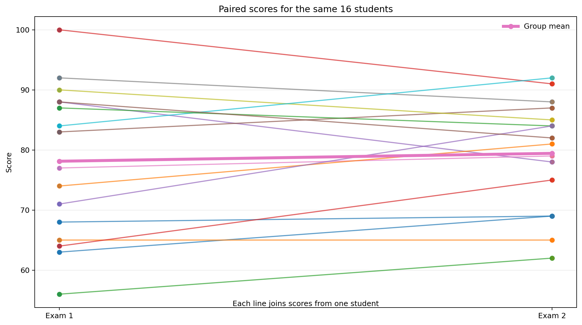
A paired line plot keeps the matching visible. Each line joins one student across the two exams. Some students improved, while others scored lower. The thick mean line shows only a small rise in the group average.
Step 2: Summarize the Difference Scores
The Exam 1 mean is 78.13 with a standard deviation of 12.66. The Exam 2 mean is 79.44 with a standard deviation of 9.15. The average difference is 1.31 points. The standard deviation of the differences is 7.00 points. There are 16 complete pairs.
| Measure | Value |
|---|---|
| Number of pairs, n | 16 |
| Exam 1 mean and standard deviation | 78.13, 12.66 |
| Exam 2 mean and standard deviation | 79.44, 9.15 |
| Mean difference, Exam 2 minus Exam 1 | 1.31 |
| Standard deviation of differences | 7.00 |
| Standard error of mean difference | 1.75 |
Step 3: Check the Difference Distribution
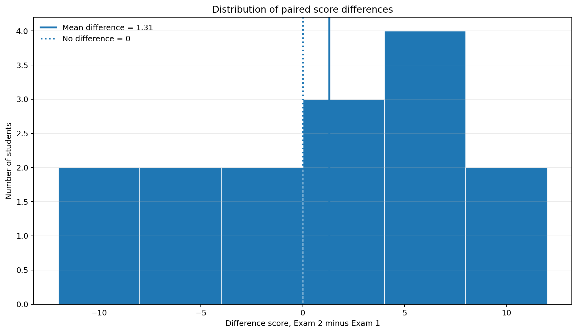
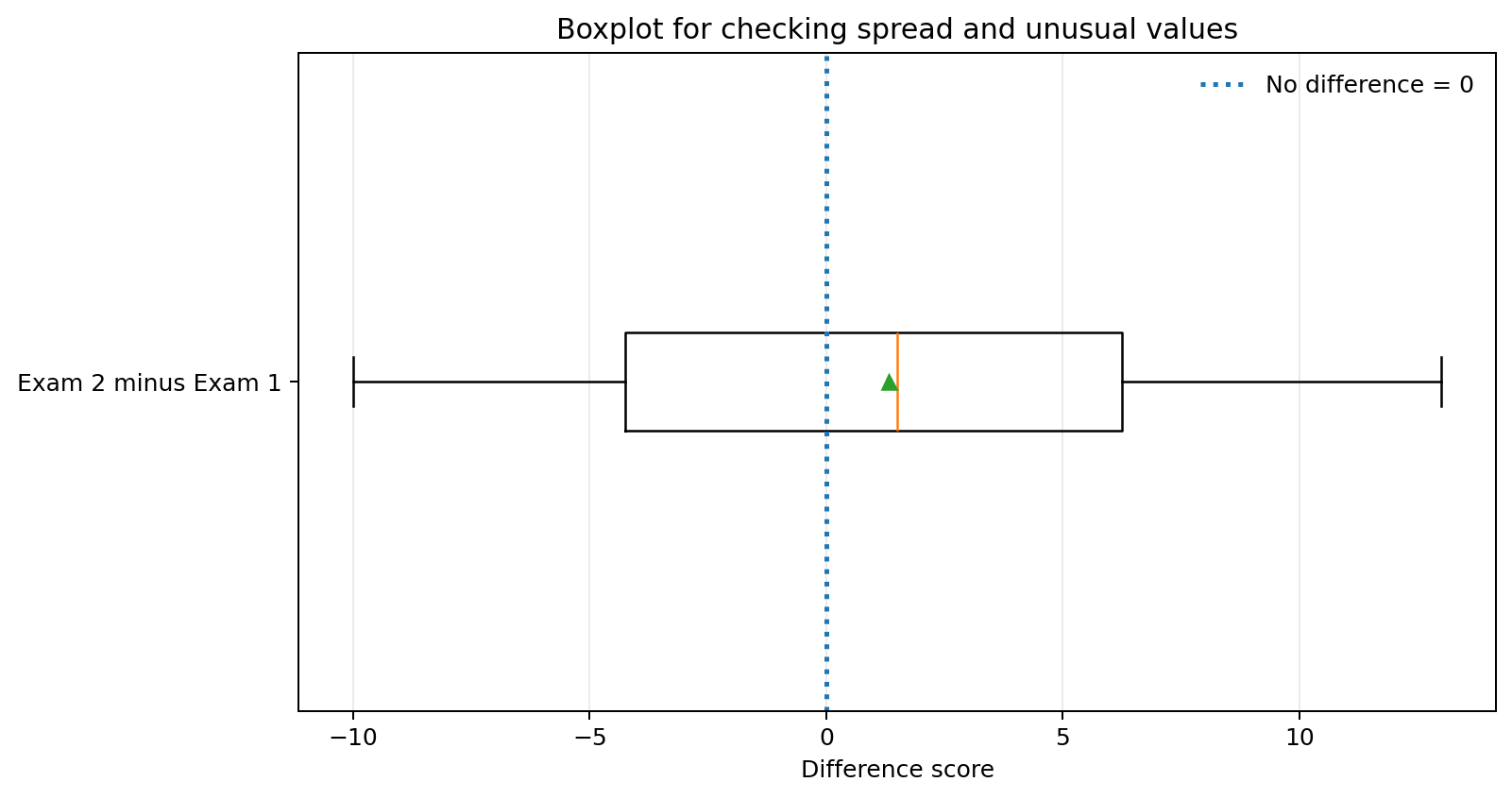
The histogram is fairly balanced for a small data set. The values range from minus 10 to 13. There is no single score far away from all others. The mean difference lies just above zero.
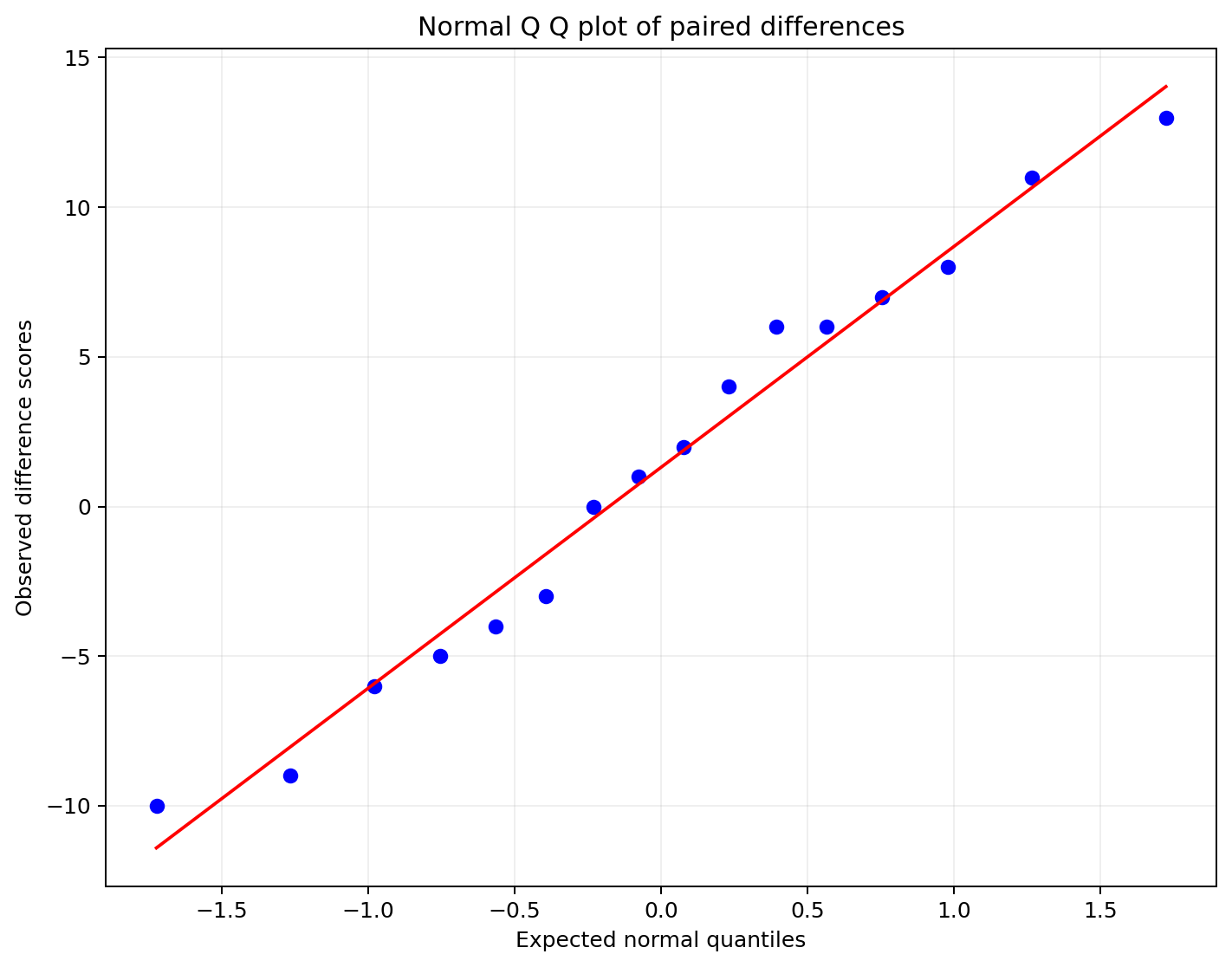
The normal Q Q plot is close to a straight line. The Shapiro Wilk result is W = .968, p = .799. This result does not show evidence against normality. The boxplot also shows no severe outlier. These checks support the use of the paired t test for this example.
Step 4: Calculate the Test Statistic
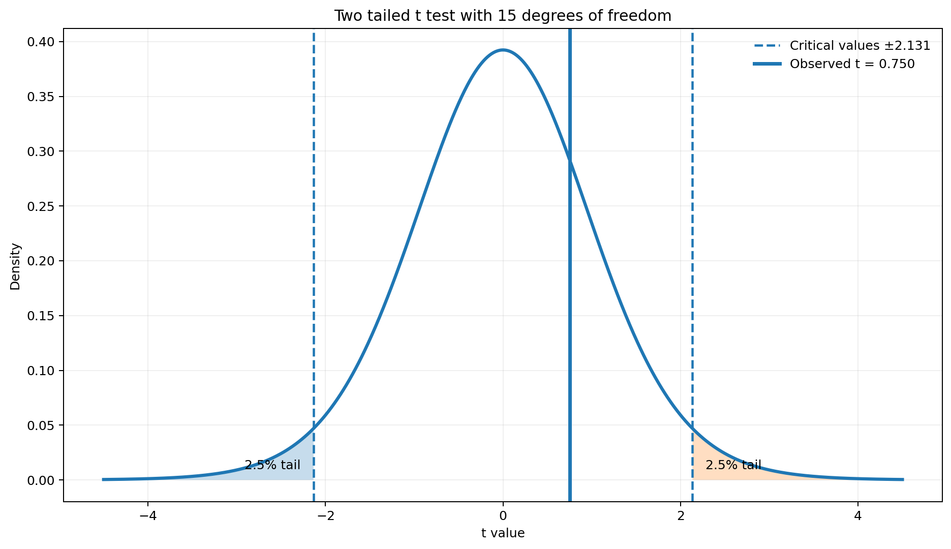
The standard error is the standard deviation of the differences divided by the square root of 16. This gives 7.002 divided by 4, or 1.751. The test statistic is the mean difference divided by that standard error.
The degrees of freedom are 16 minus 1, so df = 15. The two sided p value is .465. The 95 percent confidence interval for the mean difference is from minus 2.42 to 5.04 points.
Step 5: Make the Statistical Decision
Because p = .465 is greater than .05, we fail to reject the null hypothesis. The data do not provide strong evidence that the two exams have different mean scores. The confidence interval includes zero, which supports the same decision.
Important interpretation
A non significant result does not prove that the exams are equal. It says the study did not find clear evidence of a mean difference. If the goal is to show that two exams are close enough to be treated as equivalent, use a planned equivalence test with a meaningful margin.
How to Interpret p Values, Confidence Intervals, and Effect Size
The p Value
The p value is the probability of getting a test statistic at least as extreme as the observed one, assuming the null model is true and the test assumptions hold. It is not the probability that the null hypothesis is true. It is also not the chance that the result happened by accident.
In this example, p = .465. A result this far from zero is not unusual under a population mean difference of zero. Therefore, the sample does not give a strong reason to reject that model.
The Confidence Interval
The 95 percent confidence interval is minus 2.42 to 5.04. This range includes small negative effects, zero, and positive effects. It tells us that the estimate is not very precise. More data could narrow the interval. The interval also helps readers judge whether the possible effects matter in practice.
Cohen d for Paired Data
For paired data, one common effect size is Cohen d z. It divides the mean difference by the standard deviation of the differences. Lakens explains that this effect size has a direct link with the paired t statistic and the within subject research question [3].
The value 0.19 is small in many settings, but fixed labels such as small, medium, and large should not replace subject knowledge. Compare the effect with past research, real costs, learning goals, clinical limits, or other meaningful standards. Always state which version of Cohen d you used because several standardizers exist for repeated measures data.
APA Style Reporting Example
A good results paragraph gives the condition means and standard deviations, the test statistic, degrees of freedom, exact p value, confidence interval, and effect size. It also states the subtraction direction or describes which condition was higher.
APA style example
A paired samples t test showed that Exam 2 scores (M = 79.44, SD = 9.15) were not significantly different from Exam 1 scores (M = 78.13, SD = 12.66), t(15) = 0.75, p = .465, 95% CI [minus 2.42, 5.04], d z = 0.19. The difference was calculated as Exam 2 minus Exam 1.
Use p < .001 when the software value is smaller than .001. Otherwise, report the exact p value to three decimal places. Do not write p = .000. Report confidence interval limits with the same unit as the outcome. In a formal paper, italicize statistical symbols such as M, SD, t, p, and d according to the style guide used by your journal or university.
How to Run a Paired t Test in Statistical Software
Most software needs two equal length columns. Each row must represent one pair. Check the row order and missing data before you click run. The software may use the first column minus the second column, while your written example may use the opposite direction. Read the output labels and keep the subtraction order consistent.
SPSS Paired Samples t Test
IBM SPSS compares two variables for one group, calculates the case by case differences, and tests whether the average difference is zero. Current SPSS output can also include a confidence interval and effect size options [4].
- Place Exam 1 and Exam 2 in separate numeric columns.
- Choose Analyze, then Compare Means and Proportions, then Paired Samples t Test. Menu names can vary slightly by version.
- Move Exam 1 and Exam 2 into one pair.
- Choose Options to confirm the confidence level and missing value rule.
- Select effect size output when your version offers it.
- Read the Paired Samples Test table. Check the mean difference direction, t, df, two sided p value, and confidence interval.
T-TEST PAIRS=Exam2 WITH Exam1 (PAIRED)
  /CRITERIA=CI(.95)
  /ES DISPLAY(TRUE).
R Paired t Test
The base R t.test function uses paired = TRUE for related samples. The official R documentation states that the two vectors must have the same length and that missing values are removed in pairs [5].
exam1 <- c(63,65,56,100,88,83,77,92,90,84,68,74,87,64,71,88)
exam2 <- c(69,65,62,91,78,87,79,88,85,92,69,81,84,75,84,82)

result <- t.test(exam2, exam1, paired = TRUE,
                 alternative = "two.sided", conf.level = 0.95)
result

difference <- exam2 - exam1
mean(difference)
sd(difference)
mean(difference) / sd(difference)
Python Paired t Test
SciPy provides scipy.stats.ttest_rel for two related arrays. The current documentation returns the t statistic, p value, degrees of freedom, and a confidence interval method [6].
import numpy as np
from scipy import stats

exam1 = np.array([63,65,56,100,88,83,77,92,90,84,68,74,87,64,71,88])
exam2 = np.array([69,65,62,91,78,87,79,88,85,92,69,81,84,75,84,82])

result = stats.ttest_rel(exam2, exam1, alternative="two-sided")
difference = exam2 - exam1
cohen_dz = difference.mean() / difference.std(ddof=1)

print(result)
print(result.confidence_interval(confidence_level=0.95))
print("Cohen dz:", cohen_dz)
print("Shapiro Wilk:", stats.shapiro(difference))
Excel Paired t Test
Microsoft Excel uses T.TEST with type 1 for paired data. The tails argument is 2 for a two sided test and 1 for a one sided test [7]. If Exam 1 is in B2:B17 and Exam 2 is in C2:C17, the formula below returns the two sided p value.
=T.TEST(C2:C17,B2:B17,2,1)Excel also offers Data Analysis, then t Test: Paired Two Sample for Means, when the Analysis ToolPak is enabled. That output includes means, variances, correlation, t, critical values, and p values. Build a separate difference column to make the assumption checks and confidence interval easier.
JMP Paired t Test
JMP describes the paired t test as a test of whether the mean difference between paired measurements is zero. It also stresses that normality applies to the differences [8]. In JMP, place the two measurements in separate columns, choose Analyze, then Matched Pairs, select the two variables, and run the report. Use the difference plot and distribution tools to study assumptions.
Paired t Test vs Independent t Test vs Wilcoxon Signed Rank Test
These tests answer different questions. Choose the method from the study design and data properties, not from the p value you hope to see.
| Feature | Paired t test | Independent samples t test | Wilcoxon signed rank test |
|---|---|---|---|
| Data link | Two values are linked within each pair. | Two groups contain different units. | Two values are linked within each pair. |
| Main target | Population mean difference. | Difference between two population means. | Location shift in paired differences, often described through signed ranks. |
| Main distribution check | Approximate normality of differences. | Shape within groups, plus variance choice for the classic pooled test. | Does not require normal differences, but interpretation still needs care. |
| Typical use | Before and after values for the same people. | Treatment group compared with a separate control group. | Paired ordinal data, strong skew, or influential outliers. |
| Output | t, df, p, confidence interval, effect size. | t, df, p, confidence interval, effect size. | Rank based statistic, p value, and a suitable effect size. |
When to Use the Wilcoxon Signed Rank Test
Use the Wilcoxon signed rank test when the paired differences are strongly non normal, contain influential outliers that are valid observations, or come from an ordinal outcome where a mean is hard to defend. It ranks the absolute differences and then uses their signs. It is not simply a paired t test without assumptions. It answers a rank based question and usually works best when the difference distribution is reasonably symmetric.
For very small samples with many zero differences or strong asymmetry, consider an exact sign test, permutation test, bootstrap interval, or a model that matches the outcome scale. The right choice depends on the research question and data collection process.
Common Paired t Test Mistakes
Checking Normality on the Wrong Columns
The assumption concerns the difference scores. Exam 1 and Exam 2 can each look non normal while their differences are acceptable. Create the difference column first, then make the histogram, Q Q plot, and boxplot.
Treating Related Data as Independent
An independent t test throws away the pairing. This can reduce power and answer the wrong question. It can also give a different standard error because it ignores the within pair link.
Using the Wrong Subtraction Direction
A sign error creates confusing results. Decide whether you want after minus before or before minus after. Name the difference variable clearly and keep the same direction in tables, plots, software, and writing.
Reporting Only p < .05
A p value does not show the size of the change. Report the mean difference, confidence interval, and effect size. Readers need to know whether the result is useful, not only whether it crossed a threshold.
Calling a Non Significant Result Proof of No Difference
Failure to reject the null is not proof of equality. A wide confidence interval can hide meaningful positive or negative effects. Use equivalence testing when the goal is to show that a difference is small enough to ignore.
Deleting Outliers Without a Clear Rule
Removing valid cases can bias the result. Investigate data entry, measurement problems, and study records. Report all defensible decisions. A sensitivity analysis can show whether the conclusion changes with and without an unusual observation.
Ignoring Missing Pairs
A paired analysis needs both measurements. Count the complete pairs used by the software. Explain missing data and consider whether the missingness could be linked with the outcome.
Skipping Power and Precision Planning
A small study may miss a useful effect. Plan sample size before collecting data. Power depends on the expected standardized difference, alpha level, test direction, and number of pairs. The correlation between repeated measures can also affect the expected precision. IBM provides a paired samples power procedure in current SPSS versions [9].
A Practical Reporting Checklist
- State why the data are paired.
- Name the two measurements and the subtraction order.
- Report the number of complete pairs.
- Show means and standard deviations for both conditions.
- Show the mean and standard deviation of the differences.
- Check the difference scores with a plot and an outlier review.
- Report t, degrees of freedom, exact p value, and confidence interval.
- Report an effect size and name its formula.
- Explain the result in the original unit.
- Avoid claiming equality from a non significant test.
- Share code, data, or a clear analysis record when possible.
Frequently Asked Questions
What is a paired t test used for?
It compares the mean of two related measurements. Common examples include before and after scores, two conditions completed by the same people, and matched pairs.
What is the null hypothesis for a paired t test?
The usual null hypothesis is that the population mean difference equals zero. You can test another reference value when the research question needs it.
Do both groups need to be normally distributed?
No. The key normality check is for the paired difference scores, not each original column by itself.
Does a paired t test need equal variances?
No. The standard paired t test analyzes one set of differences, so an equal variance assumption between the two original columns is not required.
Can I use a paired t test for Likert scale data?
A total or average score built from several well designed items is sometimes treated as approximately continuous. A single ordinal item often fits a rank based method better. Explain and justify the choice.
What should I do when the differences are not normal?
Check the plots, sample size, and outliers. For strong skew or influential valid outliers, consider the Wilcoxon signed rank test, a permutation test, a robust method, or a model suited to the outcome.
What effect size should I report?
Cohen d z is common for a paired t test and uses the standard deviation of the differences. Other repeated measure effect sizes exist. State the exact formula so readers know which one you used.
How do I report a paired t test in APA style?
Report both condition means and standard deviations, t with degrees of freedom, the exact p value, a confidence interval for the mean difference, and an effect size.
Is p greater than .05 proof that the two conditions are equal?
No. It means the study did not find strong evidence of a mean difference. Use confidence intervals and an equivalence test if your goal is to support practical similarity.
What is the difference between paired and independent t tests?
A paired t test uses linked values from the same or matched units. An independent t test compares two separate groups whose observations are not linked.
Can the sample sizes in the two columns be different?
A paired t test needs one value from each condition for every included pair. Software normally removes incomplete pairs. The final paired sample size is the number of rows with both values.
When should I use a one sided paired t test?
Use it only when the direction was chosen before looking at the data and a result in the opposite direction would not count as support for the research claim.
Conclusion
The paired t test is a focused tool for two linked measurements. Its strength comes from using each pair as its own comparison. To use it well, calculate the difference scores, check their shape and unusual values, report the confidence interval and effect size, and keep the subtraction direction clear.
For the exam example, the average score rose by 1.31 points, but the evidence was not strong enough to conclude that the exams differed in mean difficulty. The result was t(15) = 0.75, p = .465, with a 95 percent confidence interval from minus 2.42 to 5.04 and Cohen d z = 0.19. This is a careful conclusion, not a claim that the exams are exactly equal.
References
[1] National Institute of Standards and Technology. Analysis of paired observations.
[2] National Institute of Standards and Technology. Normal probability plot.
[4] IBM. Paired Samples T Test, SPSS Statistics documentation.
[5] R Core Team. Student t Test, stats package documentation.
[6] SciPy Community. scipy.stats.ttest_rel documentation.
[7] Microsoft. T.TEST function documentation.
[8] JMP Statistical Discovery. Paired t Test.
Try it in DataClue
Ready to run Paired Samples t-Test?
Compare means of two related groups to assess whether their population mean differences are statistically significant.
Run Paired Samples t-Test