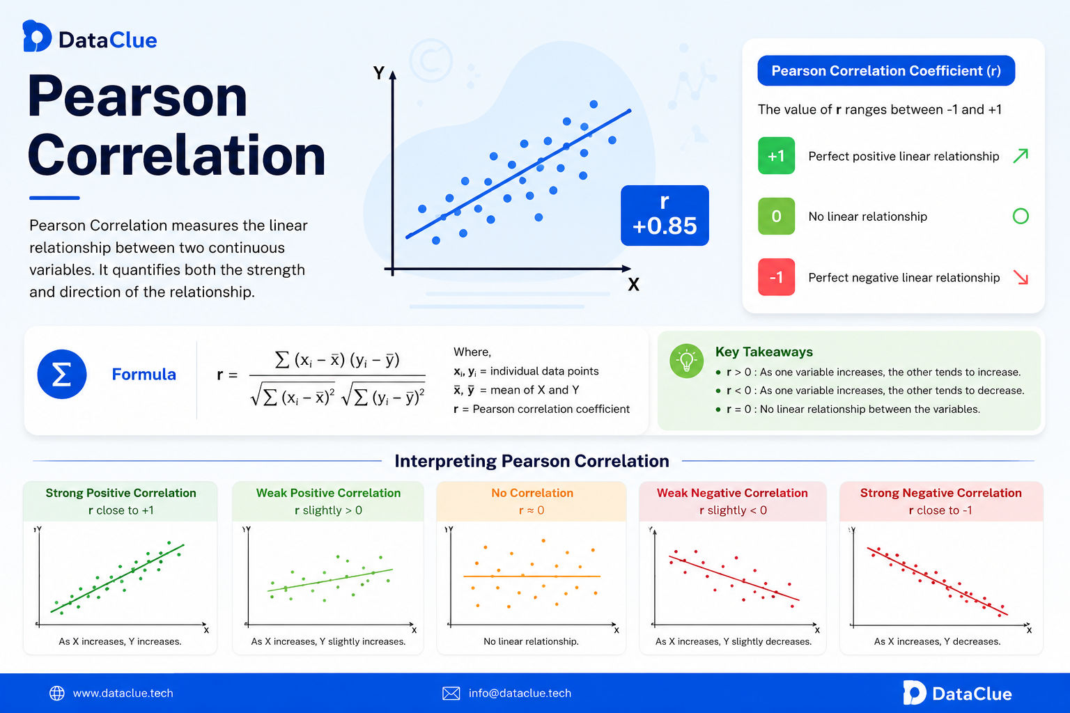
Pearson correlation is one of the most widely used statistical measures for evaluating the direction and strength of a linear relationship between two quantitative variables. It produces a coefficient, usually written as r, that ranges from -1 to +1. The sign describes the direction of the relationship, while the absolute size of the coefficient describes how closely the data follow a straight-line pattern.

Researchers, students, analysts and business teams use Pearson correlation to explore relationships such as study time and examination scores, advertising expenditure and sales, temperature and electricity consumption, or height and weight. However, the coefficient must be interpreted carefully. A high correlation does not prove causation, and a value close to zero does not necessarily mean that the variables are unrelated. It may simply mean that their relationship is nonlinear.

This guide explains the Pearson correlation formula, interpretation, assumptions, worked examples, significance testing, reporting standards, common mistakes and the main differences between Pearson, Spearman and Kendall correlation.

What is Pearson correlation?

Pearson correlation, also called the Pearson product-moment correlation coefficient, measures the degree to which two numerical variables vary together in a linear way. Each observation must contain a pair of values, one for variable X and one for variable Y. The method examines whether high values of one variable tend to occur with high or low values of the other.

A positive coefficient indicates that larger values of X are generally associated with larger values of Y. A negative coefficient indicates that larger values of X are generally associated with smaller values of Y. A coefficient close to zero indicates little evidence of a straight-line relationship, although curved or more complicated relationships may still exist.

Pearson correlation is descriptive. It summarizes the pattern in the observed sample. When combined with a confidence interval and hypothesis test, it can also be used to make an inference about the population correlation, commonly represented by the Greek letter rho (ρ).

Important: Pearson correlation describes association, not cause and effect. A third variable, reverse direction of influence, measurement error or selection bias can produce a strong correlation even when neither variable directly causes the other.

How to interpret Pearson’s r

Pearson’s r always falls between -1 and +1. The sign and magnitude should be interpreted separately:

• +1 represents a perfect positive linear relationship.
• 0 represents no linear relationship.
• -1 represents a perfect negative linear relationship.
• Values closer to +1 indicate a stronger positive linear pattern.
• Values closer to -1 indicate a stronger negative linear pattern.
• Values closer to 0 indicate a weaker linear pattern.

A perfect correlation is uncommon in real-world research because human behaviour, biological processes and business outcomes are usually influenced by many factors. Even when a relationship is meaningful, random variation and measurement error often keep r well below 1 in absolute value.

Absolute value of r	Common description	General interpretation
0.00 to 0.19	Very weak	Little linear association
0.20 to 0.39	Weak	A small linear pattern may be present
0.40 to 0.59	Moderate	A noticeable linear relationship
0.60 to 0.79	Strong	A substantial linear relationship
0.80 to 1.00	Very strong	Points closely follow a straight-line pattern

These labels are only rough guidelines. In some medical, economic or behavioural settings, a correlation of 0.20 may be practically important. In a laboratory calibration study, a correlation of 0.80 may be considered inadequate. Interpretation should therefore consider the subject area, reliability of measurement, sample size, costs and consequences of decisions.

Pearson correlation formula

The sample Pearson correlation coefficient can be written as:

r = Σ[(xᵢ - x̄)(yᵢ - ȳ)] / √[Σ(xᵢ - x̄)² × Σ(yᵢ - ȳ)²]

In the formula:

• xᵢ and yᵢ are the paired values for observation i.
• x̄ and ȳ are the sample means of X and Y.
• The numerator measures how the two variables vary together.
• The denominator standardizes the result by the variability of each variable.
• Σ indicates that the relevant quantity is summed across all paired observations.

Pearson’s r can also be described as covariance divided by the product of the standard deviations of the two variables. This standardization is why the coefficient has no units and always remains between -1 and +1. For example, changing a measurement from centimetres to metres does not change the correlation.

Worked example of Pearson correlation

Suppose a researcher records the number of hours studied and an assessment score for six students:

Student	Study hours (X)	Assessment score (Y)
A	1	52
B	2	57
C	3	65
D	4	67
E	5	75
F	6	84

The values generally increase together. Calculating Pearson’s r gives a coefficient of approximately 0.98, indicating a very strong positive linear association in this small sample. Students who studied for more hours tended to receive higher scores.

The result does not prove that additional study time alone caused the higher scores. Other variables such as prior ability, sleep, teaching quality, attendance and motivation may also influence performance. The small sample also means that the estimate is uncertain and should not be generalized without further evidence.

A good worked example should always combine the numerical result with a scatterplot, sample size, confidence interval and contextual interpretation. The coefficient by itself does not reveal whether the pattern is driven by an outlier or whether the relationship is curved.

What does r² mean?

Squaring Pearson’s r produces r², commonly called the coefficient of determination in simple linear regression. When the same two variables are used in a simple regression model, r² is the proportion of variance in the outcome that is accounted for by its linear relationship with the predictor.

For example, if r = 0.70, then r² = 0.49. In the corresponding simple linear regression, approximately 49% of the variance in the outcome is accounted for by the fitted linear relationship. The remaining 51% is not automatically “error”; it may reflect other variables, nonlinear structure, random variation and measurement limitations.

It is safer to use “accounted for by the linear model” rather than “caused by” or “explained by” when the study is observational. Correlation and regression do not establish causation without an appropriate research design and supporting assumptions.

Assumptions of Pearson correlation

Pearson correlation can be calculated for almost any two numerical variables, but meaningful interpretation and conventional inference depend on several conditions.

1. Both variables should be quantitative

Pearson correlation is designed for interval- or ratio-level measurements such as age, income, temperature, reaction time or test score. It is usually not appropriate for unordered categories. Binary variables can be handled in some special cases, but the resulting coefficient has a specific interpretation and may be better presented using methods designed for categorical data.

2. Observations must be paired correctly

Each X value must correspond to the correct Y value from the same person, object, time point or unit. Sorting one column without sorting the other destroys the pairing and produces a meaningless result.

3. The relationship should be approximately linear

Pearson’s r measures a straight-line pattern. A strong U-shaped, exponential or threshold relationship may produce a coefficient close to zero. Always inspect a scatterplot before interpreting the coefficient.

4. Observations should be independent

Repeated observations from the same participant, clustered data or time-series measurements may violate independence. Standard Pearson correlation does not adjust for these structures. Depending on the study, repeated-measures correlation, multilevel modelling, time-series methods or generalized estimating equations may be more appropriate.

5. Influential outliers should be investigated

One unusual point can increase, reduce or reverse the correlation. Outliers should not be removed simply because they are inconvenient. Check whether they result from data-entry errors, unusual but valid cases or a separate population. Report sensitivity analyses when conclusions change after an influential observation is excluded.

6. Inference requires additional distributional conditions

The coefficient itself does not require both variables to be perfectly normally distributed. Normality-related assumptions matter more for the usual p-value and confidence interval, especially in small samples. Many texts describe the classical inference model in terms of bivariate normality. With larger samples, moderate departures may be less serious, but bootstrap confidence intervals or robust methods can be useful when assumptions are doubtful.

Why a scatterplot should come before the coefficient

A single number cannot display the shape of the data. Different datasets can have the same mean, standard deviation and correlation while showing completely different patterns. A scatterplot helps identify features that Pearson’s r hides.

Before reporting the coefficient, examine the plot for:

• Curved, U-shaped or other nonlinear relationships
• Clusters that suggest subgroups or different populations
• Extreme and potentially influential observations
• Restricted range, where only a narrow part of the possible values is sampled
• Changing spread across the range of X
• Data-entry errors or impossible values
• Time trends that may create a misleading association

A correlation near zero means there is little linear association. It does not prove independence and does not rule out a strong nonlinear pattern. Similarly, a high correlation can occur because both variables increase over time, even when there is no meaningful direct relationship between them.

Pearson vs Spearman vs Kendall correlation

Pearson, Spearman and Kendall correlation answer related but different questions. The best choice depends on measurement level, shape of the relationship, ties, outliers and the purpose of analysis.

Method	What it measures	Best suited to	Main caution
Pearson r	Linear association between numerical values	Approximately linear quantitative data	Sensitive to influential outliers and nonlinear patterns
Spearman ρ	Monotonic association based on ranks	Ordinal data, skewed variables or monotonic nonlinear relationships	Does not specifically measure linearity
Kendall τ	Rank concordance between pairs	Small samples, ordinal data or many tied ranks	Often smaller numerically than Spearman correlation

A monotonic relationship consistently moves in one direction but does not need to follow a straight line. Spearman correlation can therefore be high for a curved relationship that always increases. Pearson correlation is preferable when the scientific question concerns a linear association and the measurements satisfy its conditions.

Statistical significance of Pearson correlation

A hypothesis test can evaluate whether the population correlation is zero. The usual null and alternative hypotheses are:

H₀: ρ = 0 versus H₁: ρ ≠ 0

A small p-value indicates that the observed sample correlation would be unusual under the null model. It does not show that the relationship is large, important, causal or free from bias. A very small effect may be statistically significant in a large sample, while a practically meaningful correlation may fail to reach significance in a small sample.

For a sample of n paired observations, the conventional test statistic is:

t = r√[(n - 2) / (1 - r²)], with n - 2 degrees of freedom

The test assumes that the data and sampling process are appropriate for the classical model. When assumptions are uncertain, analysts may use bootstrap intervals, permutation tests or robust correlation methods.

Confidence intervals for Pearson correlation

A confidence interval communicates the precision of the estimated population correlation. For example, r = 0.42 with a 95% confidence interval from 0.16 to 0.62 suggests a positive association but also shows uncertainty about its exact strength.

Because the sampling distribution of r is not symmetric near -1 or +1, confidence intervals are often calculated using Fisher’s z transformation. Statistical software normally performs this calculation automatically. Reports should include the interval whenever possible because a p-value alone does not show the range of plausible effect sizes.

How sample size affects correlation

Sample size affects stability and statistical power. In a small sample, the coefficient can change substantially when one observation is added or removed. Large samples provide more precise estimates but can make trivial effects statistically significant.

Required sample size depends on the smallest correlation that matters, the desired statistical power, the significance level and whether the test is one-sided or two-sided. Sample-size planning should be completed before data collection whenever correlation is a primary analysis.

Common applications of Pearson correlation

Pearson correlation is used across many disciplines, including:

• Education: study time and examination performance
• Healthcare: age and blood pressure, or dosage and response under suitable conditions
• Psychology: scores from two validated measurement scales
• Finance: returns of two assets over the same time periods
• Marketing: advertising expenditure and sales revenue
• Operations: production volume and energy consumption
• Environmental research: temperature and measured demand
• Quality control: readings from two measurement instruments

In each application, the paired measurements, design and assumptions must be checked. Correlations based on aggregated groups can differ from correlations among individuals, a problem related to ecological fallacy. Time-series and financial return data may also contain autocorrelation, nonstationarity or volatility patterns that require specialized methods.

Common mistakes when using Pearson correlation

Confusing correlation with causation. A strong association does not show that changing X will change Y. Experimental design, temporal order, confounding control and subject-matter reasoning are needed for causal claims.

Ignoring outliers. One influential observation can create an impressive coefficient or hide a genuine relationship. Always compare the result with the scatterplot and consider sensitivity analysis.

Using Pearson correlation for a nonlinear relationship. A low value may occur even when the variables have a strong curved association. Consider transformation, nonlinear modelling or a rank-based method when scientifically appropriate.

Reporting only the p-value. Readers need the coefficient, sample size, confidence interval, scatterplot and practical interpretation.

Applying universal strength labels. Thresholds such as 0.30 or 0.50 should not replace field-specific judgement.

Correlating many variables without adjustment. Testing a large correlation matrix increases the chance of false-positive findings. Pre-specify important comparisons or apply a suitable multiple-testing procedure.

Ignoring missing data. Software may use different subsets of observations for different correlations. State whether complete-case or pairwise deletion was used and assess whether missingness could bias the result.

Restricting the range. Sampling only high-performing students or a narrow age group can reduce the observed correlation compared with the broader population.

How to calculate Pearson correlation

Most spreadsheet and statistical programs calculate Pearson’s r quickly. Before using any command, confirm that the two columns are aligned, missing values are handled consistently and the scatterplot supports a linear interpretation.

Excel or Google Sheets

Use the CORREL function with two equal-length ranges:

=CORREL(A2:A101, B2:B101)

Excel also provides PEARSON, which produces the same coefficient. The spreadsheet result does not automatically provide a p-value or confidence interval, so additional calculations or statistical software may be needed for complete reporting.

Python with SciPy

The pearsonr function returns the coefficient and a two-sided p-value:

from scipy.stats import pearsonr r, p_value = pearsonr(x, y)

Check the documentation for the installed SciPy version when using confidence intervals or alternative hypotheses, because software interfaces can change.

R

The cor.test function reports the correlation, test statistic, degrees of freedom, p-value and confidence interval:

cor.test(x, y, method = "pearson")

SPSS

Choose Analyze > Correlate > Bivariate, move the relevant variables into the analysis box, select Pearson and choose the required significance test. Review the output together with a scatterplot and descriptive statistics.

How to report Pearson correlation

A complete report should name the variables, state the direction and strength of the association, provide r, sample size or degrees of freedom, confidence interval and p-value, and briefly discuss whether assumptions were checked.

Example APA-style report:

Study time was positively correlated with assessment score, r(48) = .42, 95% CI [.16, .62], p = .002. The scatterplot indicated an approximately linear relationship with no clearly influential outliers.

The number in parentheses is the degrees of freedom, calculated as n - 2 for the conventional test. Therefore, r(48) corresponds to a sample of 50 paired observations.

For a non-significant result, avoid saying that there is “no relationship.” Instead, report the estimate and interval. For example, an interval from -0.10 to 0.38 indicates that the data remain compatible with effects ranging from a small negative association to a moderate positive association.

How to improve the reliability of a correlation analysis

• Define the research question and analysis plan before examining the results.
• Use reliable, valid and appropriately scaled measurements.
• Collect a sample that represents the population of interest.
• Inspect distributions and scatterplots before calculating the coefficient.
• Investigate missing values, outliers and possible data errors transparently.
• Report effect size and uncertainty, not only statistical significance.
• Run sensitivity analyses when conclusions depend on a few observations.
• Distinguish exploratory findings from pre-specified confirmatory analyses.
• Use subject-matter knowledge to interpret practical importance.

  Summary

  Pearson correlation is a compact and useful measure of linear association between two quantitative variables. Its coefficient ranges from -1 to +1, with the sign indicating direction and the magnitude indicating how closely the observations follow a straight-line pattern. A responsible analysis goes beyond calculating r: it checks the scatterplot, assumptions, outliers, sample size and uncertainty.

  Use Pearson correlation when the variables are numerical, correctly paired and approximately linearly related. Consider Spearman or Kendall correlation for ranks, ordinal data or monotonic relationships that are not linear. Report the coefficient with its sample size, confidence interval, p-value and contextual meaning, and avoid interpreting association as causation.

Frequently asked questions

What is considered a strong Pearson correlation?

There is no universal cutoff. Values above 0.70 are often called strong, but importance depends on the field, measurement reliability, sample and consequences of the decision. A smaller coefficient may be meaningful in complex human or public-health outcomes.

When should I avoid Pearson correlation?

Avoid or reconsider it when the variables are not meaningfully quantitative, the relationship is clearly nonlinear, observations are dependent, the sample contains highly influential outliers, or the research question concerns ranks or ordinal responses rather than numerical distances.

Does Pearson correlation require normally distributed variables?

The coefficient can be calculated without normality. The classical p-value and confidence interval rely on stronger assumptions, particularly in small samples. Inspect the data and consider bootstrap, permutation or robust approaches when distributional conditions are doubtful.

Can Pearson correlation be used for Likert-scale data?

A single Likert item is ordinal, so Spearman or Kendall correlation is often easier to justify. Researchers sometimes treat multi-item scale totals as approximately continuous when the scale is well constructed and has enough distinct values, but the choice should be explained.

What does a negative Pearson correlation mean?

A negative value means that higher values of one variable tend to be associated with lower values of the other. The closer the coefficient is to -1, the stronger the negative linear pattern.

Can Pearson correlation be greater than 1?

No. A valid Pearson correlation must lie between -1 and +1. A result outside this range indicates a calculation, coding or data-processing error.

What does r = 0 mean?

It means there is no linear association in the observed sample. The variables may still have a nonlinear relationship, so the scatterplot remains essential.

Is Pearson correlation affected by units?

No. Because the coefficient is standardized, converting kilograms to grams or metres to centimetres does not change r, provided the transformation is positive and linear.

How many observations are needed?

There is no single minimum that guarantees a reliable result. The required sample depends on the expected effect, desired precision, statistical power and data quality. Small samples produce unstable coefficients and wide confidence intervals.

What is the difference between correlation and regression?

Correlation treats the variables symmetrically and summarizes their linear association. Regression specifies an outcome and one or more predictors, estimates a fitted equation and can support prediction or adjusted analysis under appropriate assumptions.

Can a high correlation still be misleading?

Yes. A high value may result from an outlier, common time trend, restricted sampling, duplicated data, confounding or aggregation. Always examine the study design and the underlying observations.

Should I use a one-tailed or two-tailed test?

A two-tailed test is the usual default because it allows either a positive or negative population correlation. A one-tailed test should be chosen only when a directional hypothesis was justified before observing the data and an effect in the opposite direction would not support the claim.

updated on 15-08-2026