What Is a Regression Model? Types, Analysis, and Examples

A regression model is a statistical and machine-learning method that estimates how a target variable relates to one or more predictors. It can explain patterns in existing data and predict numerical outcomes such as prices, sales, demand, costs, production time, or energy use.

A useful model does more than draw a best-fit line. It needs an appropriate target, relevant data, realistic validation, suitable error metrics, and careful interpretation. A model may fit historical observations closely and still fail when the operating environment, customer population, or data collection process changes.

What Is a Regression Model in Simple Terms?

A regression model estimates the relationship between a target variable and one or more predictor variables. It can be used to describe conditional associations or to predict numerical outcomes for new observations.

Suppose a factory manager wants to estimate how many worker hours will be needed for a production order. The number of units is a predictor, and worker hours are the target. Regression uses earlier production records to estimate how labor tends to change as production volume changes.

Dependent variables and independent variables

The value being estimated is commonly called the dependent variable, response, outcome, label, or target. The inputs are called independent variables, explanatory variables, predictors, features, regressors, or covariates. “Target” and “feature” are common in machine learning, while “dependent variable” and “explanatory variable” are common in statistics and econometrics.

Prediction, explanation, and association

Regression serves different goals. Predictive modeling asks how accurately an outcome can be estimated for unseen cases. Explanatory modeling asks how the outcome changes with a predictor while other included variables are held constant. Causal inference asks what would happen if an intervention changed that predictor. A fitted coefficient usually supports an association; it does not prove causation without a defensible design and additional assumptions.

Why Regression Models Matter in 2026

Many practical decisions concern quantities rather than classes. Organizations forecast revenue, inventory demand, delivery time, asset values, customer lifetime value, energy consumption, hospital resource use, and staffing requirements. Linear regression also remains a useful baseline because it is quick to train, easy to audit, and capable of revealing whether a more complicated method adds meaningful value.

Google’s current machine-learning material presents linear regression as a method for predicting a numerical label from features and describes training as adjusting model parameters to reduce prediction loss.^[1] This simple framework still underpins more advanced workflows involving regularization, feature engineering, cross-validation, and production monitoring.

The practical reality is that interpretability, data availability, maintenance effort, and decision cost often matter as much as a leaderboard score. A transparent model that is slightly less accurate may be preferable when analysts must explain a forecast, audit its inputs, or update it with limited resources.

How a Regression Model Works

The workflow begins with historical observations containing known target values and candidate predictors. The model estimates parameters that connect the predictors to the target, produces fitted values, and measures the difference between each fitted value and the observed outcome.

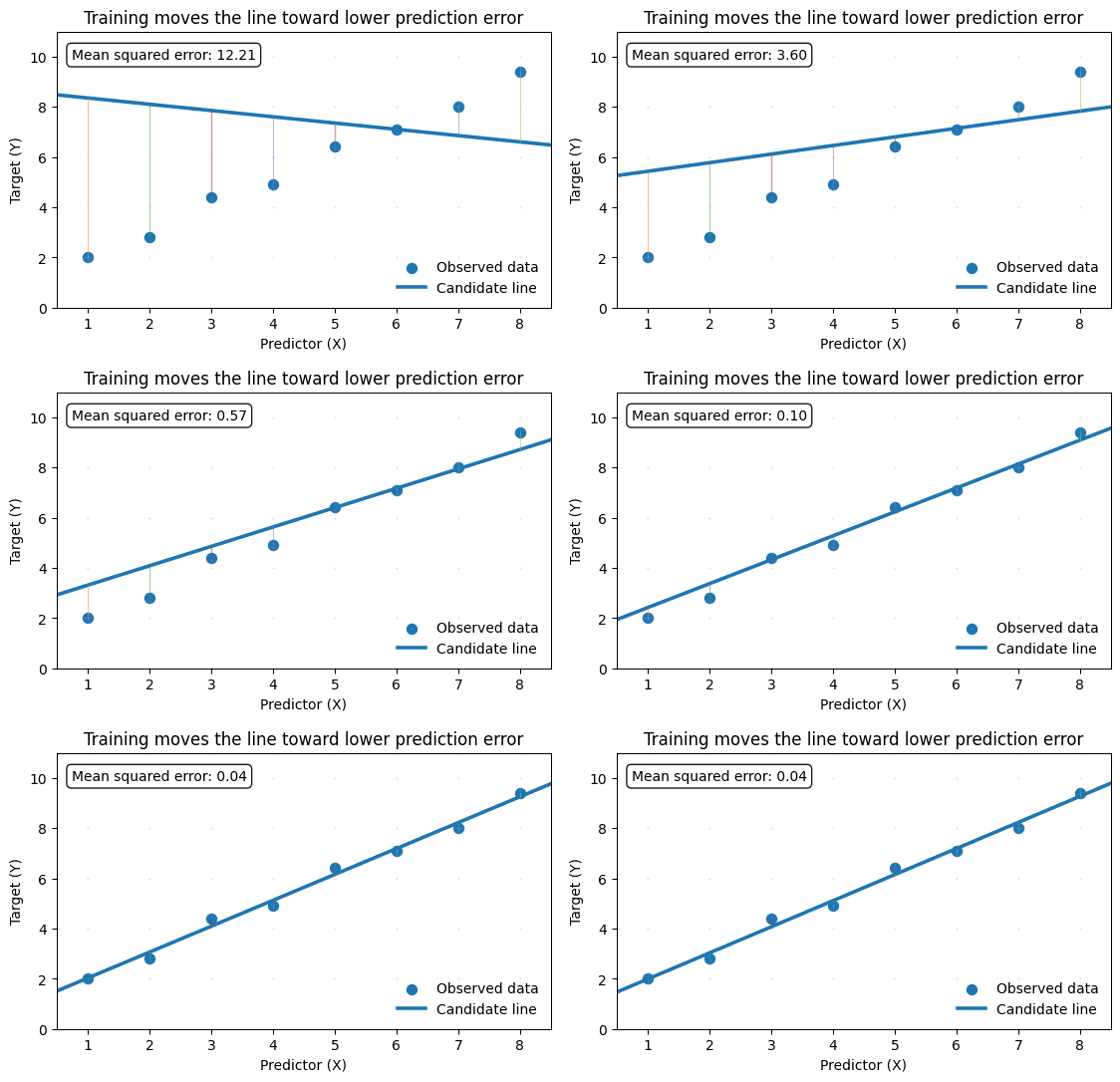
For ordinary least squares, the coefficients are chosen to minimize the sum of squared residuals. A residual is the observed value minus the fitted value. Squaring residuals prevents positive and negative errors from cancelling and gives larger misses more influence on the fitted line.^[2]

After training, the same equation can estimate the target for a new combination of predictor values. That estimate is useful only if the new case is sufficiently similar to the data and conditions used to develop the model.

What Is the Regression Equation?

Simple linear regression formula

Y is the target, X is the predictor, a is the intercept, b is the slope or coefficient, and u is the unobserved error term. The fitted version replaces the unknown population parameters with estimates and produces a predicted value.

Multiple linear regression formula

Multiple linear regression includes two or more predictors. Each coefficient describes the estimated change in the target associated with a one-unit increase in that predictor while the other included predictors are held constant.

How to interpret a coefficient

Consider the fitted equation “sales = 20,000 − 800 × price + 2.4 × advertising spend.” The price coefficient suggests that a one-unit price increase is associated with 800 fewer units of sales when advertising is unchanged. The advertising coefficient suggests 2.4 additional sales units for each unit of advertising spend when price is unchanged. These are conditional associations within the model, not guaranteed causal effects.

The intercept is the predicted target when all numerical predictors equal zero and categorical predictors are at their reference levels. It should not be given a real-world story automatically. Zero may be impossible, outside the observed range, or simply irrelevant to the decision.

What Are the Main Types of Regression Models?

Simple and multiple linear regression

Simple linear regression uses one predictor. Multiple linear regression uses several predictors and can represent more realistic systems, although adding variables does not automatically improve the model. Irrelevant, leaked, or poorly measured features can make results less stable and harder to maintain.

Polynomial and nonlinear regression

Polynomial regression adds terms such as X² or X³ to represent curvature. It is still linear in its coefficients even though the fitted relationship is curved. Nonlinear regression instead fits a function that is nonlinear in its parameters, often based on a known growth, decay, saturation, or physical process. Both approaches require caution because flexible curves can follow noise and behave implausibly outside the observed range.

Ridge, Lasso, and Elastic Net

Ridge regression adds an L2 penalty that discourages large coefficients and can stabilize estimates when predictors are strongly correlated. Lasso adds an L1 penalty and can shrink some coefficients to zero, creating a sparse model. Elastic Net combines both penalties and is often useful when many predictors carry overlapping information. Scikit-learn notes that Elastic Net can retain groups of correlated features more reliably than Lasso, which may select one of them somewhat arbitrarily.^[2]

Stepwise, robust, and quantile regression

Stepwise regression adds or removes predictors according to a selection rule, but repeated selection can produce unstable coefficients and overly confident inference. Robust regression reduces the influence of extreme residuals, while quantile regression estimates a conditional quantile such as the median instead of the conditional mean. These methods solve different problems and should not be treated as automatic upgrades.

Logistic regression

Logistic regression estimates the probability of a categorical outcome, usually through a sigmoid function. In machine-learning workflows it is treated as a classification method, whereas linear regression predicts continuous numerical values.^[3]

Regression Model Types Compared

Regression type	Best used for	Main characteristic	Typical output
Simple linear	One main predictor	Straight-line relationship	Continuous value
Multiple linear	Several predictors	Conditional effects within one equation	Continuous value
Polynomial	Curved patterns	Adds powers of predictors	Continuous value
Ridge	Correlated predictors	L2 coefficient shrinkage	Continuous value
Lasso	Sparse feature sets	L1 penalty can set coefficients to zero	Continuous value
Elastic Net	Many correlated features	Combines L1 and L2 penalties	Continuous value
Logistic	Binary or multiclass targets	Estimates class probability	Probability or class
Nonlinear	Known complex response shapes	Fits a specified nonlinear function	Continuous value

The right method depends on the target, relationship shape, sample structure, prediction cost, and need for interpretation. The most sophisticated algorithm is not automatically the most suitable one.

Linear Regression vs Logistic Regression

Decision factor	Linear regression	Logistic regression
Target	Continuous numerical outcome	Categorical outcome
Raw output	Numerical prediction	Probability between zero and one
Example	Predicting monthly revenue	Predicting customer churn
Typical evaluation	MAE, RMSE, R²	Log loss, precision, recall, ROC-AUC
Fitted form	Linear combination of features	Probability curve based on a linear score

Choose linear regression when the outcome is a measurable quantity. Choose logistic regression when the outcome represents a category such as churn or no churn. Although logistic regression returns probabilities, it is trained using categorical outcomes and is normally evaluated as a classifier.

When Should You Use Regression Analysis?

Regression is appropriate when the outcome is measurable, the historical data contains relevant predictors, and the relationship is stable enough to support the intended explanation or forecast. The predictors must also be available at the moment the prediction will be made.

Suitable questions include how much inventory a store will need, how long an order will take, how property features relate to sale price, how temperature affects electricity demand, and how price or advertising is associated with sales. In SaaS and e-commerce, regression can estimate customer lifetime value, order value, demand, or support workload. It is less suitable when the target is purely categorical, the available features carry little signal, or the process changes faster than the model can be maintained.

When regression is the wrong method

A standard regression model may fail when important predictors are missing, records are not comparable, the relationship changes sharply over time, or the analysis depends on extreme extrapolation. It is also insufficient when the main goal is to establish causation. Causal questions require a research design and assumptions that address confounding, timing, selection, measurement, and alternative explanations.

What Assumptions Matter in Linear Regression?

Assumptions should not be treated as a memorized pass-or-fail checklist. Different violations affect different parts of the analysis. Some mainly weaken p-values and confidence intervals, while others damage coefficient stability, prediction quality, or the meaning of the model itself.

Linearity and model form

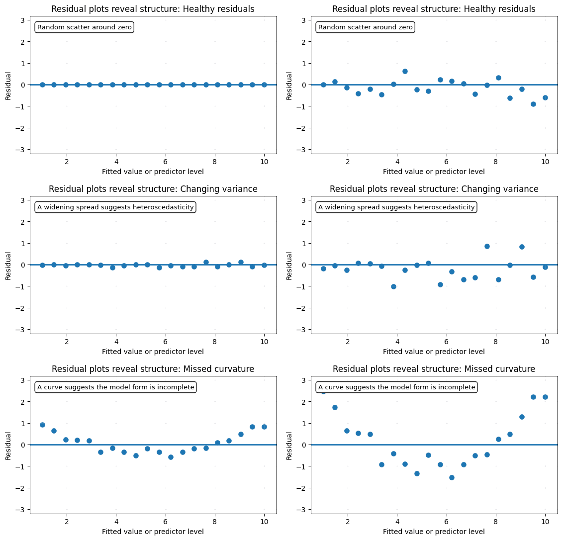
The conditional mean of the target should be represented adequately by the chosen equation. Curved residual patterns may indicate missing nonlinear terms, interactions, transformations, or an unsuitable algorithm.

Independence of errors

Errors should not contain unexplained dependence. Dependence is common in time series, repeated customer records, households, classrooms, production batches, and geographic data. A random split that places related observations in both training and testing sets may create an unrealistically optimistic result.

Homoscedasticity and residual normality

Homoscedasticity means that residual variance is approximately constant across the fitted range. A widening funnel suggests heteroscedasticity. Normality generally concerns residual errors for classical inference, not a requirement that every raw predictor and target variable follow a bell curve. NIST describes classical regression errors as normally and independently distributed around zero with constant variance.^[4]

Multicollinearity and influential observations

Predictors do not need to be completely independent. The practical problem is severe multicollinearity, which can make individual coefficients unstable even when predictions remain acceptable. Unusual observations may also exert strong influence because of a large residual, an extreme predictor value, or both. Statsmodels provides residual, leverage, influence, heteroscedasticity, and variance-inflation diagnostics for investigating these issues.^[5][9]

How Do You Evaluate a Regression Model?

Evaluation should use data that did not train the model. Training performance shows how closely the model learned its existing sample; it does not establish how well the model will generalize to future cases.

MAE, MSE, and RMSE

Mean Absolute Error measures the average absolute distance between actual and predicted values. Mean Squared Error squares each error, so large misses receive disproportionately more weight. Root Mean Squared Error takes the square root of MSE, returning the result to the target’s original units while preserving the stronger penalty on large errors.^[6]

R-squared and adjusted R-squared

R² compares the model with a mean-based reference. A value near one indicates a strong fit for that evaluation set. A value of zero is comparable to predicting the mean, and a negative value means the model performed worse than that reference. A high R² does not prove causation, reliable future performance, or operational usefulness.^[6]

Adjusted R² penalizes predictors that do not contribute enough explanatory value. It is useful when comparing related linear models fitted to the same outcome, but it is not a substitute for testing on unseen data.

MAPE and its zero-value problem

Mean Absolute Percentage Error expresses errors relative to actual values, which can be convenient across different scales. It becomes unstable when actual values are zero or close to zero, so it should not be selected merely because percentages appear easy to explain.^[6]

Metric	What it emphasizes	Preferred direction	Main limitation
MAE	Typical absolute error	Lower	Does not strongly penalize rare large errors
MSE	Squared error	Lower	Not expressed in the target’s original units
RMSE	Large errors in target units	Lower	Sensitive to extreme errors
R²	Improvement over a mean reference	Higher	Can hide unacceptable practical errors
Adjusted R²	Fit adjusted for predictor count	Higher	Mainly an in-sample linear-model measure
MAPE	Relative percentage error	Lower	Unreliable near zero

Why metric choice can change the decision

Imagine that Model A makes errors of 4, 4, 4, and 4 units, while Model B makes errors of 0, 0, 0, and 9 units. Model A has an MAE of 4 and an RMSE of 4. Model B has a better MAE of 2.25 but a worse RMSE of 4.5. Model B is preferable when typical error matters most; Model A is preferable when one large failure is especially costly.

This is why a model should be judged against the decision it supports. A delivery forecast, medical resource plan, or cash-flow estimate may need an asymmetric or domain-specific cost function rather than a generic score.

Cross-validation and realistic splitting

Cross-validation estimates how performance varies across repeated training and validation splits. It supports model comparison and tuning, but the splitting strategy must match the data. Time-ordered forecasting needs time-aware validation, while repeated records may require grouped splits. Scikit-learn describes cross-validation as an estimate of a range of expected generalization scores, not a guarantee of future performance.^[7]

How to Build a Regression Model

Define the decision question

Start with the decision, prediction horizon, and acceptable error. “Predict sales” is vague. “Predict weekly unit sales for each store four weeks ahead so inventory can be ordered” defines a target, time horizon, unit of analysis, and practical use.

Choose a measurable target

The target must be consistently recorded and aligned with the real objective. Predicting clicks is not the same as predicting profitable sales, and predicting revenue is not the same as predicting contribution margin.

Select predictors available at prediction time

Candidate features should be plausible, measurable, and available before the outcome occurs. Information recorded after the outcome creates data leakage and can make a weak model look highly accurate.

Clean and explore the data

Check missing values, duplicates, units, category labels, impossible values, recording changes, time trends, and unusual observations. Plot the target against important predictors. This work often reveals that the main problem is data definition rather than algorithm choice.

Create realistic training, validation, and test sets

The final test set should represent the cases the model will face. Keep future periods out of training for forecasting. Keep related records together when customers, patients, properties, or production batches would otherwise leak across the split.

Establish a baseline and train an interpretable first model

Compare the model with a simple rule such as predicting the training mean, median, last observed value, or seasonal average. Ordinary linear regression is often an effective first benchmark. A more complex model should earn its additional cost by improving realistic validation performance or solving a documented limitation.

Evaluate, diagnose, and improve

Calculate decision-relevant metrics on unseen data, inspect individual errors, and review residual plots. Improvements may include corrected data, transformations, interactions, regularization, robust methods, or a nonlinear algorithm. Tune choices with validation data rather than repeatedly consulting the final test set.

Deploy and monitor

Document the data period, feature definitions, transformations, model version, validation results, known limitations, and intended action. After deployment, monitor errors, input distributions, missingness, extreme predictions, subgroup performance, and changes in the relationship between predictors and outcomes.

How to Interpret Regression Results

Coefficients and the “holding constant” condition

A coefficient estimates how the predicted target changes with a one-unit increase in that predictor while other included predictors remain constant. Units and transformations matter. A coefficient for dollars cannot be compared directly with one for percentages or standardized scores without considering scale.

P-values, confidence intervals, and practical importance

A p-value addresses a statistical null hypothesis under the model assumptions. A small p-value does not prove a large, useful, or causal effect. Confidence intervals describe uncertainty in an estimated parameter. Practical importance depends on the size of the effect, its uncertainty, implementation cost, and the decision threshold.

Prediction intervals vs confidence intervals

A confidence interval for the mean response expresses uncertainty about the average outcome at specified predictor values. A prediction interval for a new observation is wider because it also includes individual outcome variation. Statsmodels supports separate interval calculations for mean predictions and new observations.^[8]

Correlation does not establish causation

A strong coefficient can reflect direct influence, reverse causality, a shared cause, selection effects, or measurement choices. Causal language requires a design and analysis that address these alternatives rather than relying on statistical significance alone.

Real-World Regression Model Examples

Property valuation

A property model may use floor area, neighborhood, building age, condition, bedroom count, and market conditions. Geography is not a decorative keyword: local supply, transport access, regulations, and market cycles can change the relationship. A model trained in one city or country should not be assumed to generalize to another without validation.

Sales, e-commerce, and SaaS forecasting

Sales models may use price, promotion, advertising, season, product availability, economic conditions, and previous sales. E-commerce teams may estimate order value or demand, while SaaS teams may model customer lifetime value or support workload. Targets must be defined carefully: gross revenue, retained revenue, and profit represent different business questions.

Manufacturing and staffing

Production volume, product type, machine availability, setup time, shift, and worker experience may help predict labor hours. The model may fail near capacity limits because overtime, machine constraints, or bulk efficiencies change the relationship.

Finance and economics

Regression can estimate historical relationships among asset returns, market factors, interest rates, inflation, or economic activity. A historical coefficient such as market beta describes sensitivity over the fitted period; it does not guarantee that the relationship will persist.

Healthcare and other high-stakes settings

Regression can estimate length of stay, resource use, or measured outcomes, but high-stakes applications need representative data, privacy controls, subgroup analysis, uncertainty reporting, and domain-expert review. Predictive accuracy alone does not establish clinical suitability or fairness.

Regression Analysis Example With Calculation

Consider a factory with the following observed production data.

Units produced	Worker hours
10	32
20	49
30	71
40	88
50	110

The least-squares fitted equation is:

The slope means that each additional unit is associated with about 1.95 additional worker hours within the conditions represented by the sample. At 35 units, the prediction is 11.5 + 1.95 × 35 = 79.75 hours.

At 30 units, the fitted value is 70 hours and the observed value is 71, so the residual is 1 hour. That residual shows the part of the observation not captured by the line.

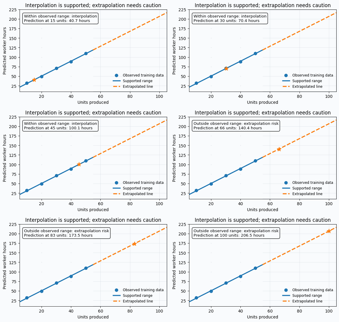
The same equation predicts 206.5 hours for 100 units, but 100 is far outside the observed range of 10 to 50. The factory may encounter capacity limits, additional shifts, supply shortages, or scale efficiencies. The arithmetic is valid; the real-world assumption is weak.

Common Regression Mistakes and Risks

Confusing association with causation

A coefficient is not an intervention effect by default. Unsupported causal language is one of the most serious interpretation errors because it can turn a useful descriptive model into misleading advice.

Ignoring data quality and feature timing

A sophisticated algorithm cannot repair a target that was recorded inconsistently. Features available only after the target occurs create leakage and may produce excellent test scores that disappear in actual use.

Adding too many predictors

More features can improve training fit while increasing variance, multicollinearity, maintenance effort, and leakage risk. Each feature should have a clear domain, predictive, or inferential purpose.

Using R² as the only verdict

R² can look impressive while typical errors remain too large, particular groups perform poorly, or the model fails after the environment changes. Always connect evaluation to the operational decision.

Ignoring residual patterns and influential observations

Aggregate metrics can hide curvature, changing variance, clusters, and unusual cases. Investigate why an observation is influential before removing it. The unusual case may be a data error, a legitimate rare event, or the exact failure the system must handle.

Overfitting and extrapolation

An overfitted model learns noise and performs poorly on new data. Extreme extrapolation is a separate risk: even a stable model may be asked to predict where it has no evidence. Simpler features, regularization, realistic validation, and explicit prediction boundaries help control these risks.

How to Improve a Regression Model

The largest gains often come from improving the question and data rather than replacing the algorithm. Correcting the target, collecting a missing predictor, preventing leakage, or using the right split may matter more than extensive hyperparameter tuning.

Transformations can help when effects are multiplicative, residual variance grows with the target, or relationships are curved. Interaction terms represent situations in which the effect of one feature depends on another. Ridge, Lasso, and Elastic Net can control complexity, while robust regression can reduce the influence of genuine but extreme residuals.

A nonlinear model should be adopted only when it produces a meaningful improvement on realistic unseen data and the additional learning curve, compute cost, explanation burden, and maintenance effort are justified. The realistic goal is not maximum complexity; it is dependable performance at an acceptable operational cost.

How AI Tools Can Support Regression Analysis

Generative tools such as ChatGPT and Gemini can explain terminology, draft Python or R code, suggest visualizations, and convert output into plainer language. AI agents or AutoML systems can automate feature processing, model comparison, and tuning when their workflow is configured correctly.

Their limitation is not merely occasional coding error. AI-generated analysis may use the wrong target, a leaking feature, an unrealistic split, an unsuitable metric, or causal language unsupported by the design. A script can execute successfully while the underlying analysis remains invalid.

Use generative models as assistants for code, documentation, and diagnostic ideas. Keep responsibility for data meaning, validation design, assumption checking, high-stakes suitability, and final interpretation with qualified human reviewers.

Regression in Statistics vs Machine Learning

Statistical regression often emphasizes coefficients, uncertainty, hypothesis tests, and assumptions about the data-generating process. Machine-learning regression often emphasizes predictive performance on unseen data, cross-validation, regularization, feature pipelines, deployment, and monitoring.

The distinction is one of emphasis rather than a rigid boundary. A strong practical analysis can combine both traditions: validate predictions realistically, inspect failure modes, report uncertainty, and interpret coefficients only within the assumptions the data can support.

The conventional rule that the model with the highest score is best is therefore incomplete. A useful model must also be stable, maintainable, understandable at the required level, affordable to operate, and connected to an action that improves the decision.

FAQs

What is the main purpose of regression?

Regression is used to estimate conditional relationships and predict outcomes from observed data. The exact purpose should be stated as prediction, explanation, or causal analysis because those goals require different evidence.

What is the difference between regression and correlation?

Correlation summarizes the strength and direction of association between variables. Regression defines a target, estimates a conditional relationship, and can generate predictions.

Does regression prove causation?

No. Regression alone identifies modeled associations. Causal claims require a suitable research design and assumptions that address confounding and alternative explanations.

What is the simplest regression model?

Simple linear regression uses one predictor to estimate a continuous target through a straight-line relationship.

Can R-squared be negative?

Yes. On evaluation data, R² can be negative when the model performs worse than a mean-based reference prediction.^[6]

Is logistic regression a regression or classification model?

In most machine-learning workflows, logistic regression is a classifier because it estimates probabilities for categorical outcomes.^[3]

Can regression handle nonlinear data?

Yes. Polynomial features, specified nonlinear functions, regression trees, boosting, support vector regression, and other methods can model nonlinear patterns.

Which software is used for regression analysis?

Common options include Python with scikit-learn or statsmodels, R, SPSS, SAS, Stata, Excel, and MATLAB. The best choice depends on whether the priority is teaching, inference, automation, or deployment.

How much data does a regression model need?

There is no universal minimum. The requirement depends on predictor count, noise, effect size, dependence among records, model complexity, subgroup needs, and the accuracy required for the decision.

Regression Model Checklist

Stage	What should be confirmed
Before modeling	The decision, target, prediction horizon, population, acceptable error, and available predictors are clearly defined.
Data preparation	Missingness, duplicates, units, category definitions, timing, and leakage risks have been reviewed.
Model development	A simple baseline exists, the split reflects real use, and model choices are evaluated on unseen data.
Diagnostics	Residual patterns, multicollinearity, influential observations, subgroup errors, and uncertainty have been examined.
Before deployment	Inputs will be available in production, limitations are documented, and the prediction leads to a defined action.
After deployment	Performance, drift, missingness, extreme outputs, and retraining conditions are monitored.

Choosing a Regression Model You Can Trust

A regression model converts observed relationships into a predictive or explanatory function, but mathematical fit is only the beginning. The model must match the target, use information available at prediction time, perform acceptably on realistic unseen data, and communicate uncertainty honestly.

Start with a clear decision question and a simple baseline. Select the model according to the target and data structure, choose metrics that reflect the cost of errors, inspect residuals, and avoid unsupported causal conclusions. Use a more complex method only when it solves a documented problem and its additional effort is justified.

The most trustworthy model is rarely the one with the highest R² or the largest number of features. It is the simplest approach that remains accurate enough, stable enough, and useful enough under the conditions in which people will actually rely on it.

References

1. Google for Developers, “Linear regression”

2. scikit-learn, “Linear Models”

3. Google for Developers, “Logistic Regression”

4. NIST/SEMATECH, “Check of assumptions”

5. statsmodels, “Linear regression diagnostics”

6. scikit-learn, “Metrics and scoring”

7. scikit-learn, “Cross-validation: evaluating estimator performance”

8. statsmodels, “OLSResults.get_prediction”

9. statsmodels, “Regression diagnostics”