Sample Size Calculator & Research Guide

A sample size calculator helps determine how many participants, responses, observations, cases, or experimental units a study needs. For a simple survey estimating a population proportion at 95% confidence, a ±5 percentage-point margin of error, and an assumed proportion of 50%, the familiar large-population result is about 385 completed responses. That number is useful, but it is not a universal sample size for research. [1]

The correct calculation depends first on the research question. If the goal is to estimate a percentage, prevalence, or mean with specified precision, use a precision-based sample size method. If the goal is to detect a difference, association, intervention effect, correlation, or regression effect, use a design-specific power analysis. Choosing the method before choosing the number is the central rule of sound sample size planning.

Calculate Your Sample Size

For a standard survey or descriptive study estimating a population proportion, the calculator below needs the confidence level, desired margin of error, expected population proportion, and, when the population is finite, the population size. The HTML version of this guide includes an interactive calculator that also adjusts for design effect and expected retention or response rate.

Calculator inputs for the interactive HTML version

Population size	Optional; leave effectively unlimited for a very large population
Confidence level	95%
Margin of error	5%
Expected proportion	50%
Design effect	1.0
Expected usable response / retention	100%
Default result	385 usable responses

The Word version is static. The accompanying HTML file contains the working calculator with finite-population, design-effect, and retention adjustments.

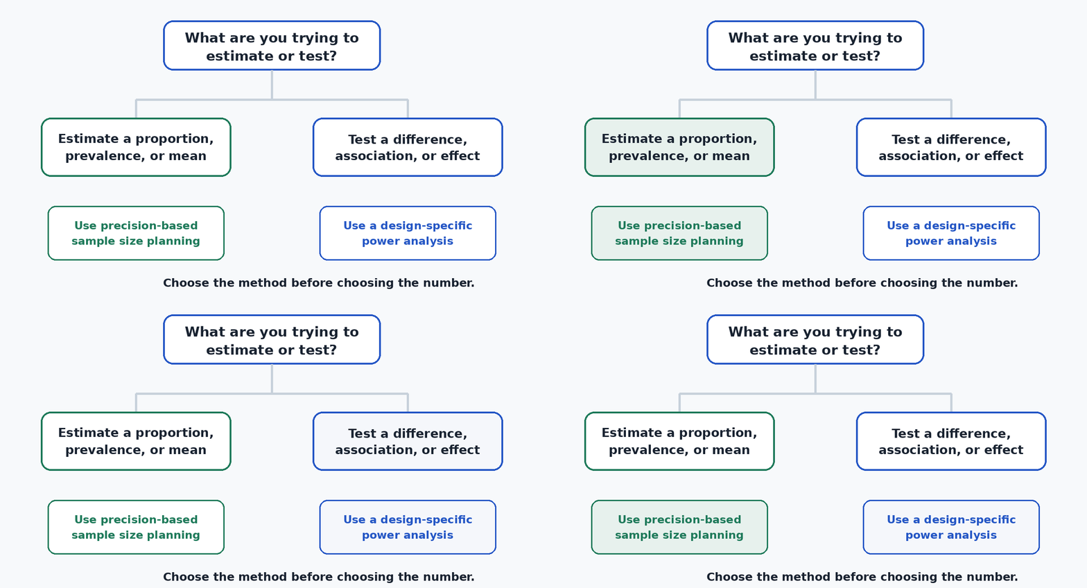
Start with the research objective. Estimation and hypothesis testing require different sample size logic.

Sample Size Calculator for Surveys and Proportion Studies

The standard large-population calculation for a proportion is n₀ = Z²p(1-p)/e². If the population is finite, apply a finite population correction before multiplying by any design effect. Finally, adjust the resulting analytic requirement for expected nonresponse, attrition, or unusable data. [1][3][4]

Input	What it means	Common starting point
Population size, N	The number of eligible units in a clearly defined finite population	Leave effectively unlimited when N is very large relative to the sample
Confidence level	Controls the confidence-interval procedure and its critical value	95% is common, not mandatory
Margin of error, e	The desired half-width around a proportion estimate	±5 percentage points is common for general surveys
Expected proportion, p	Expected prevalence or proportion with the characteristic	0.50 when no defensible estimate exists
Design effect	Variance inflation from a complex sampling design	1.0 for simple random sampling
Retention/response rate	Expected fraction of recruited or invited cases that remain usable	Use study-specific evidence when possible

Quick decision rule: Use a precision formula when the main objective is estimating a proportion or mean. Use power analysis when the main objective is testing a difference, relationship, or effect. A four-field survey calculator cannot determine the sample required for every research design.

What Sample Size Means and Why It Matters

Sample Size in Simple Terms

Sample size is the number of independent units contributing usable information to an analysis. Depending on the study, a unit might be a person, household, school, company, patient, experimental animal, laboratory specimen, transaction, or another experimental unit. The word participant is therefore not always interchangeable with observation.

Population, Sample, and Sampling Frame

The target population is the group to which the research question refers. The accessible population is the part of that group that can realistically be sampled. The sampling frame is the operational list or mechanism used to select units. The sample is the subset actually observed. These distinctions matter because a mathematically adequate sample drawn from a poor frame can still produce biased conclusions.

Planned, Recruited, Completed, and Analytic Samples

A planned sample size is the target determined before data collection. A recruitment or invitation target is usually larger because some people will not respond, will withdraw, or will provide unusable data. The completed sample is the number who finish the study, while the analytic sample is the number whose data are included in the primary analysis. A strong methodology section reports these stages clearly rather than treating them as one number.

How Sample Size Affects Precision and Statistical Power

For estimation, larger samples usually reduce standard errors and narrow confidence intervals. For hypothesis testing, larger samples usually increase statistical power for a specified effect. Small samples can therefore leave estimates too imprecise or make meaningful effects hard to detect. Very large samples can be wasteful when the extra precision or power adds little practical value.

A Large Sample Cannot Fix a Bad Sampling Process

Sample size addresses how much information is collected under a set of assumptions. It does not correct coverage bias, convenience sampling, systematic nonresponse, misleading questions, measurement error, poor outcome definitions, or a statistical model that does not match the research question. CDC guidance for population-survey sample size explicitly assumes a random or representative sample. [3]

Risk warning: A mathematically adequate sample size does not make a biased or nonrepresentative sample valid. Precision and representativeness are different properties.

What Information Do You Need to Calculate Sample Size?

Population Size

Population size, N, is most important when sampling without replacement from a finite population and the required sample represents a meaningful fraction of that population. There is no universal population cutoff such as 100,000 below which a finite population correction suddenly becomes necessary. The relevant issue is the sampling fraction: how large n is relative to N. [1]

Confidence Level and Z-Score

A confidence level specifies the long-run coverage of the interval procedure. Common two-sided normal critical values are approximately 1.645 for 90%, 1.96 for 95%, and 2.576 for 99%. A 95% confidence interval is not best interpreted as a 95% probability that a fixed population parameter lies inside the one interval already calculated. Rather, the interval-producing procedure has 95% long-run coverage under its assumptions.

Margin of Error and Precision

For a proportion estimate, the margin of error is the desired half-width of the confidence interval. In the basic formula, required n is proportional to 1/e². This means halving the margin of error requires roughly four times the sample when other inputs are unchanged. [1]

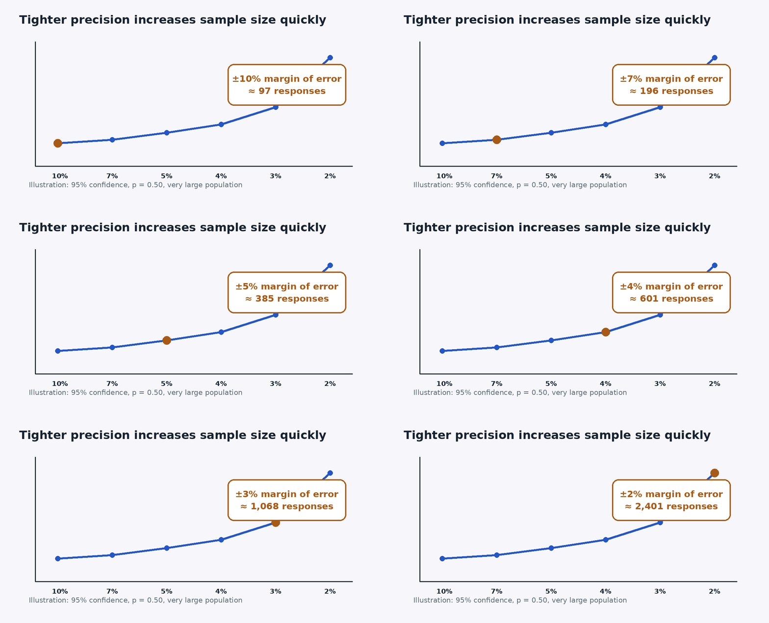
Tighter precision is expensive in sample size. At fixed confidence and p = 0.50, halving the margin of error roughly quadruples the required sample.

Population Proportion

For a binary outcome, p is the expected proportion with the characteristic of interest. When no defensible prior estimate exists, p = 0.50 is commonly used because p(1-p) reaches its maximum at 0.50. That choice produces the largest sample under the basic proportion formula and is therefore conservative with respect to the unknown proportion. [1]

Standard Deviation for Estimating a Mean

If the objective is to estimate a population mean rather than a proportion, the calculation needs an anticipated standard deviation, σ, and a desired margin in the original measurement units. A common planning approximation is n = (Zσ/E)², rounded upward. Penn State gives the same relationship for confidence intervals around a mean. [2]

Effect Size, Alpha, and Statistical Power

Power-based studies require a plausible effect size, a significance level α, and desired power 1-β. Effect size might be expressed as Cohen’s d, Cohen’s f, f², a correlation coefficient, an odds ratio, a raw mean difference, or another quantity matched to the planned test. Smaller effects generally require larger samples when alpha and power are held constant.

Effect-size assumptions should come from the strongest relevant evidence available, such as a meta-analysis, well-designed prior studies, carefully interpreted pilot data, or a minimum effect that would matter scientifically or practically. Changing the effect size simply to produce an affordable sample undermines the logic of a priori planning.

Groups, Predictors, Repeated Measurements, and Clusters

More complex designs need more than a single effect size. Two-group studies need an allocation ratio. Regression analyses need the inferential target and predictor structure. Repeated-measures analyses depend on within-person correlations and covariance assumptions. Cluster and multilevel designs depend on cluster size and intracluster similarity. These design parameters can materially change the effective amount of information in a nominal sample.

How to Calculate Sample Size for a Survey

Cochran-Style Sample Size Formula for a Proportion

For a large population and a proportion outcome, the standard precision formula is:

n₀ = Z² × p × (1 − p) / e²

Here, n₀ is the initial required sample, Z is the critical value for the chosen confidence level, p is the expected population proportion, and e is the desired absolute margin of error. Penn State presents this same large-population formulation. [1]

Worked Example: 95% Confidence and ±5% Margin of Error

Using Z = 1.96, p = 0.50, and e = 0.05:

n₀ = (1.96² × 0.50 × 0.50) / 0.05² = 384.16

Round the final result upward, giving a minimum of 385 usable observations under the stated assumptions.

Why 385 Appears So Often

The number 385 is common because 95% confidence, ±5 percentage-point precision, p = 0.50, and an effectively large population are common defaults. It is not the minimum sample size for quantitative research and it should not be carried automatically into experiments, regression, correlation, factor analysis, structural equation modeling, clustered surveys, or qualitative interviews.

Large-population assumptions	Approximate required N
90% confidence, ±5%, p = 0.50	271
95% confidence, ±5%, p = 0.50	385
99% confidence, ±5%, p = 0.50	664
95% confidence, ±3%, p = 0.50	1,068
95% confidence, ±2%, p = 0.50	2,401

When a Smaller p Produces a Smaller N

If credible prior evidence suggests p is far from 0.50, the basic formula can produce a smaller sample. That does not automatically mean the resulting study will be useful. For a rare outcome, an absolute margin of error of ±5 percentage points may be much too wide relative to the prevalence itself. The precision target must be scientifically meaningful, not merely convenient.

Finite Populations, Nonresponse, and Attrition

Finite Population Correction

When sampling without replacement from a known, finite population, an initial large-population result can be adjusted using:

n = n₀ / [1 + (n₀ − 1) / N]

The correction matters most when n is not small relative to N. Penn State’s sampling guidance derives finite-population sample-size formulas directly and shows how ignoring the correction can substantially overstate the required sample in small populations. [1]

Worked Example for a Population of 1,000

Keep the unrounded large-population value n₀ = 384.16 and apply the correction:

n = 384.16 / [1 + 383.16 / 1,000] = 277.74 → 278

A calculator that rounds 384.16 to 385 before applying the correction may return 279 instead. That one-person difference is a rounding artifact. A cleaner implementation preserves full numerical precision internally and rounds the final required sample upward.

Worked Example for a Population of 1,200

n = 384.16 / [1 + 383.16 / 1,200] = 291.18 → 292

Why a Population of One Million Does Not Require Thousands of Responses

Once the population is very large relative to the required sample, further increases in N barely change the precision of a simple random sample of fixed size. With 95% confidence, ±5% precision, and p = 0.50, the requirement is about 278 for N = 1,000, about 370 for N = 10,000, about 383 for N = 100,000, and about 385 for a population of one million or more.

Minimum Analytic Sample vs Recruitment Target

A formula normally gives the number of usable observations needed for analysis. Recruitment planning asks how many people must be invited or enrolled to end with that number. The adjustment is:

Recruitment target = required analytic sample / expected retention or response proportion

Example: Allowing for 20% Loss

If 385 usable cases are required and 20% of recruited cases are expected to be lost, the expected retention is 0.80:

385 / 0.80 = 481.25 → recruit 482

Simply adding 20% gives 462, but losing 20% of 462 leaves only about 370 usable cases. Dividing by the retention rate is the correct arithmetic for a planned loss fraction.

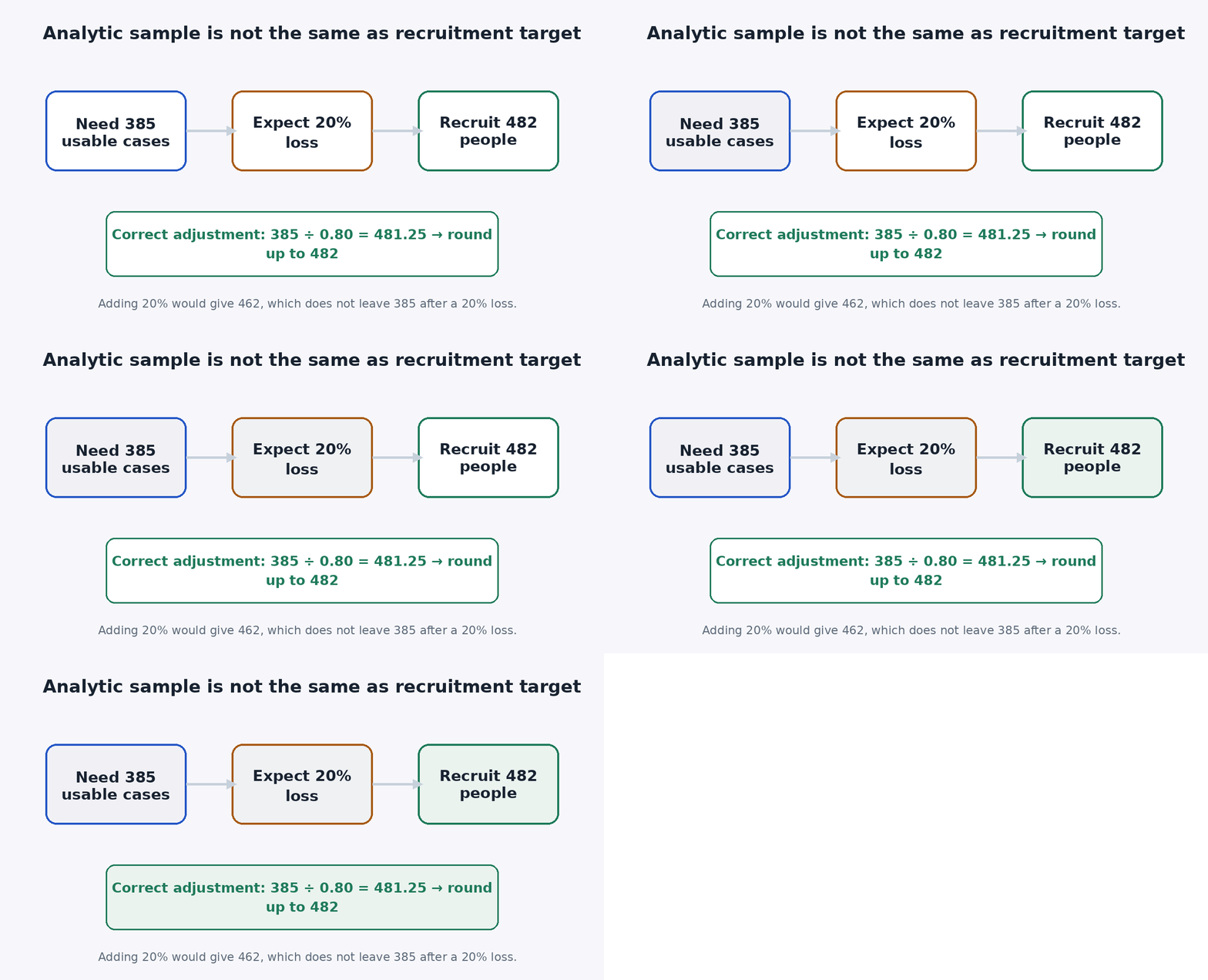
Recruitment targets should be inflated by dividing by the expected retention or response proportion.

Nonresponse Is Also a Bias Problem

Recruiting more people can protect the final sample count, but it does not automatically fix nonresponse bias. If the people who do not respond differ systematically from those who do, the final estimate may remain biased even when the numerical target is reached. Quantity and representativeness must be managed separately.

Which Sample Size Method Should You Use?

The best method follows the primary estimand or hypothesis. The table below is a routing guide, not a substitute for design-specific planning.

Research objective	Preferred planning approach	Key inputs
Estimate a population proportion or prevalence	Confidence interval / precision calculation	Confidence level, desired precision, expected p, finite N if relevant
Estimate a population mean	Precision calculation for a mean	Confidence level, desired margin in outcome units, expected SD
Compare two or more groups	Power analysis for the planned test	Effect size, alpha, power, group allocation
Test a correlation	Power analysis for correlation	Expected r, alpha, power, one- or two-sided test
Multiple regression inference	Power analysis matched to the model test	Effect size, alpha, power, predictors or tested parameters
Prediction model development	Model-specific sample-size criteria	Predictor parameters, outcome prevalence, anticipated model performance
Repeated or longitudinal outcomes	Design-specific power analysis	Effect, repeated-measure correlation/covariance, time points, attrition
Clustered or multilevel data	Design-effect, multilevel, or simulation approach	Clusters, cluster size, intracluster correlation, effect
Factor analysis / SEM	Model-specific or simulation-based planning	Loadings, communalities, indicators, factors, paths, missingness
Qualitative interviews	Information adequacy / information power	Study aim, sample specificity, theory, dialogue quality, analytic strategy

Descriptive Surveys and Prevalence Studies

Use a precision-based proportion calculation when the primary objective is to estimate a binary characteristic such as prevalence, support, adoption, or satisfaction to a specified absolute precision. If the survey uses clustering, unequal selection probabilities, or complex weighting, the simple random sample formula may understate variance and must be adjusted. [3][4]

Complex, Clustered, and Multilevel Designs

Cluster sampling often yields less independent information than the same number of independently sampled individuals because people within a cluster tend to resemble one another. CDC guidance recommends building an expected design effect into sample-size planning for cluster surveys. [4]

A common approximation is DEFF = 1 + (m − 1)ρ, where m is average cluster size and ρ is the intracluster correlation. This shows why increasing the number of clusters can be more informative than simply adding more individuals within the same clusters when within-cluster similarity is high.

Subgroup Analysis and Oversampling

An overall sample can be adequate for the population estimate yet too small for meaningful subgroup estimates. If conclusions about age groups, regions, professions, treatment strata, or other subgroups are primary, size those comparisons or subgroup precision targets explicitly. Stratification or oversampling may be needed, with appropriate weighting at analysis when selection probabilities differ.

Qualitative Research

A margin-of-error calculator is not an appropriate way to determine the number of qualitative interviews. Malterud and colleagues proposed information power as a planning framework: the more relevant information the sample provides for the study aim, the fewer participants may be needed. Sample specificity, use of theory, dialogue quality, and analysis strategy all matter. [9]

How to Calculate Sample Size With G*Power

What G*Power Does

G*Power is a statistical power-analysis program maintained by researchers at Heinrich Heine University Düsseldorf. The official site states that it supports many t tests, F tests, chi-square tests, z tests, and some exact tests, and can also compute effect sizes and display power-analysis results graphically. [5]

Start With the Statistical Question, Not the Software Menu

First identify the primary hypothesis and the statistical test that will answer it. “Does an intervention improve outcomes?” may imply an independent-groups comparison, repeated-measures interaction, mixed model, or another test depending on the design. Selecting the wrong G*Power procedure can produce a numerically precise answer to the wrong question.

Choose an A Priori Analysis

For prospective planning, use an a priori analysis. Specify the effect size, alpha, desired power, and relevant design inputs; the program then solves for the required N. The G*Power documentation and foundational papers describe this relationship between effect size, alpha, power, and sample size. [5]

Choose an Evidence-Based Effect Size

The effect-size assumption should be justified before the sample is calculated. Prefer a relevant meta-analysis or strong previous research when available. Pilot data can help, but estimates from small pilots are unstable. Another defensible approach is to define the smallest effect that would still change a scientific, clinical, policy, or business decision.

Use Sensitivity Analysis When the Effect Is Uncertain

One number can create false certainty when the effect size is poorly known. Calculate several plausible scenarios, such as a conservative effect, the best-supported effect, and an optimistic effect. If a modest change in effect size causes a large jump in required N, that uncertainty is part of the feasibility decision and should be documented.

Adjust for Attrition After the Power Calculation

The N returned by an a priori power analysis is usually the required analytic sample under the entered assumptions. Inflate recruitment separately for anticipated attrition, incomplete data, exclusions, or unequal allocation when those are not already built into the design calculation.

Sample Size for Common Statistical Tests and Complex Models

Independent-Samples t-Test

Planning an independent-samples t-test requires the standardized or raw mean difference of interest, variability, alpha, desired power, sidedness, and group allocation. For illustration, a two-sided comparison with Cohen’s d = 0.50, alpha = .05, power = .80, and equal groups requires roughly 128 participants in total under standard calculations, about 64 per group. This is an illustration, not a rule for every two-group study.

Paired-Samples t-Test

Paired designs use within-person or matched differences. The required N depends on the variability of those differences, which in turn depends on the relationship between paired measurements. Because each participant serves as their own reference, a paired design can be more efficient than an independent-groups design when the pairing is strong and the design is appropriate.

One-Way ANOVA

ANOVA planning depends on the number of groups, the effect-size definition, alpha, power, and the hypothesis being tested. Changing the number of groups or targeting specific contrasts can change the requirement. Treat any example such as “about 159 for three groups at f = .25, alpha = .05, power = .80” as conditional on those exact assumptions, not as an ANOVA standard.

Correlation

Correlation sample size depends on the smallest correlation worth detecting, alpha, desired power, and whether the test is one- or two-sided. A study designed for r = .30 can require far fewer cases than one designed for r = .10. That is why “100 participants for a correlation” is not a generally defensible rule.

Multiple Regression and Prediction Models

For regression inference, the correct calculation depends on whether the target is the overall model, an increase in R², or a specific predictor conditional on others. Prediction-model development is a different objective again. Riley and colleagues show that prediction-model sample size should consider overfitting, anticipated model performance, outcome frequency, and the number of predictor parameters rather than relying on a fixed participants-per-predictor or events-per-variable rule. [6]

Logistic Regression and Rare Outcomes

When a binary outcome is rare, the number of outcome events can become the limiting resource. The historical “10 events per variable” heuristic is not a universal requirement. Modern prediction-model guidance shows that required events per predictor can be below or well above 10 depending on the anticipated model and desired protection against overfitting. [6]

Mediation and Moderation

Indirect effects and interactions are often harder to detect than simple main effects. The necessary sample depends on the component paths, reliability, distributional assumptions, and the inferential method. Simulation or specialized power tools are often more appropriate than applying a generic regression rule.

Factor Analysis

Fixed ratios such as “10 participants per item” are easy to remember but incomplete. MacCallum and colleagues showed that factor-analysis sample requirements depend on characteristics such as communalities and factor overdetermination. A clean model with strong loadings can behave differently from a weak or ambiguous factor structure at the same N-to-item ratio. [7]

Structural Equation Modeling

SEM has no single defensible minimum such as 200 cases. Simulation work by Wolf and colleagues found large differences in required N across models as factor loadings, path coefficients, indicators, factors, and missingness changed. Their simulations produced acceptable sample sizes ranging from roughly 30 to 460 under the model conditions examined, illustrating why fixed rules can both overestimate and underestimate requirements. [8]

Sample Size Rules of Thumb and Method Comparisons

Is 385 Always the Right Sample Size?

No. Approximately 385 is the large-population answer for one proportion-estimation scenario: 95% confidence, ±5 percentage-point precision, and p = 0.50. It is not a universal benchmark for research.

Is a Sample Size of 30 Enough?

There is no general rule that n = 30 makes a study representative, adequately powered, or statistically valid. Thirty may be enough for some narrowly defined large-effect or pilot objectives and far too small for others. The analysis and decision target determine adequacy.

Cochran-Style Formula vs Slovin’s Formula vs G*Power

Method	Question it answers	Strength	Main limitation
Cochran-style proportion formula	How many observations are needed to estimate a proportion with specified precision?	Makes confidence, p, and precision explicit	Not a general hypothesis-testing calculator
Finite population correction	How much can the sample be reduced when sampling a finite population without replacement?	Uses the relationship between n and N	Requires a meaningful finite accessible population
Slovin/Yamane-style shortcut	What sample follows from N and an error term under restrictive assumptions?	Simple and quick	Hides assumptions and is often used outside its valid context
G*Power	How many observations are needed to detect a specified effect with a particular test?	Test-specific power framework	Depends on justified effect-size and design inputs
Simulation-based planning	How does a complex model perform across candidate sample sizes?	Can reflect model-specific assumptions	Requires greater statistical skill and setup

The formula commonly labeled Slovin’s, n = N/(1 + Ne²), is frequently applied as though it were a universal survey formula. Tejada and Punzalan examined its misuse and argued that its interpretation is much narrower, corresponding to specific assumptions rather than arbitrary sampling problems. [11]

When Rules of Thumb Are Useful

Rules of thumb can support early feasibility discussions when little design information exists. They should not become the final justification when the primary analysis can be planned directly. A useful rule is one that prompts a more precise calculation, not one that replaces it.

A Practical Contrarian Point: Bigger Is Not Always the First Fix

When a study appears weak, the instinct is often to increase N. Sometimes that is correct. In other situations, improving the sampling frame, reducing measurement error, clarifying the primary outcome, balancing allocation, increasing the number of clusters, or simplifying an overambitious model can improve the study more than adding participants indiscriminately. Sample size controls quantity, not whether the design answers the right question.

How to Choose and Report a Defensible Sample Size

Start With the Primary Research Question

Write the primary question in a form that makes the statistical objective explicit. Are you estimating a population quantity, testing a difference, evaluating an association, developing a prediction model, or exploring qualitative experiences? That decision determines the appropriate planning framework.

Define the Primary Outcome or Estimand

A study may collect dozens of variables, but sample-size planning should be anchored to the main quantity the study must estimate or the main hypothesis it must test. Planning around a secondary outcome while leaving the primary objective underpowered creates a mismatch between the stated purpose and the design.

Document Every Assumption

For precision-based calculations, document confidence, precision, p or SD, N if finite, and the sampling design. For power analysis, document the statistical test, effect size and its source, alpha, power, allocation, and other design parameters. Then show how nonresponse, dropout, or exclusions altered the recruitment target.

Sample Size Justification for a Survey

A concise methodology paragraph can state: “Sample size was determined for estimation of a population proportion using a 95% confidence level, a five-percentage-point margin of error, and p = 0.50 because no sufficiently reliable prior estimate was available. The large-population calculation yielded n = 384.16, which was rounded upward to a minimum analytic sample of 385. The recruitment target was adjusted separately for anticipated nonresponse.” Add finite-population or design-effect adjustments when they apply.

Sample Size Justification for a Power Analysis

A power-analysis paragraph can state: “An a priori power analysis was conducted for the primary [statistical test]. Assuming [effect size and source], alpha = [value], desired power = [value], and [groups/predictors/allocation], the analysis indicated a minimum analytic sample of [N]. The recruitment target was increased to [N] to allow for an anticipated [x%] loss.” Every bracketed value must be replaced with the study’s own justified assumptions.

Report Planned and Achieved Samples Separately

After data collection, report how many people were invited or assessed for eligibility, how many were enrolled, how many completed the study, and how many entered the primary analysis. If the final analytic N differs from the plan, report the deviation transparently rather than recalculating the original rationale to match what happened.

Common Sample Size Mistakes and Troubleshooting

Choosing the Sample Before Choosing the Statistical Test

Starting with an available number such as 100, 200, or 385 and then searching for a justification reverses the planning process. Define the research objective and analysis first, calculate the requirement second, and then evaluate feasibility.

Treating Margin of Error as Total Research Error

A ±5% sampling margin does not bound all sources of research error. It does not include coverage error, measurement error, nonresponse bias, coding mistakes, model misspecification, or other nonsampling errors.

Ignoring Complex Sampling

If respondents are sampled within schools, clinics, villages, households, workplaces, or other clusters, a simple-random calculation can overstate the effective information. Cluster design and weighting should be incorporated into planning and analysis. [4]

Using an Unsupported Effect Size

Effect size is often the most influential assumption in a power analysis. Copying a “medium” Cohen convention without asking whether that effect is realistic or meaningful can produce a sample that is statistically tidy but scientifically weak. Conventions are fallback benchmarks, not evidence about a particular research problem.

Why Two Sample Size Calculators Give Different Answers

Two tools can disagree because one applies finite-population correction and another does not, one rounds intermediate values, p values differ, confidence critical values differ, one includes a design effect, one adjusts for losses, or one reports per-group rather than total N. Compare assumptions before deciding that a calculator is wrong.

Using Post Hoc Power to Explain a Nonsignificant Result

Observed post hoc power calculated from the study’s observed effect is generally not informative for interpreting completed-study results. Heinsberg and Weeks demonstrate why it is closely tied to the observed data and can mislead researchers about whether a nonsignificant result reflects low true power. Confidence intervals and the range of effects compatible with the data are usually more informative after the study is complete. [10]

What If You Already Know the Maximum Sample You Can Collect?

Reverse the planning question instead of manipulating assumptions. For an estimation study, calculate the precision achievable with the feasible N. For a hypothesis-testing study, calculate the minimum detectable effect at the feasible N, alpha, and desired power. This sensitivity analysis tells you what the study can realistically learn.

For example, with n = 220, p = 0.50, 95% confidence, and a very large population, the approximate sampling margin is about ±6.6 percentage points under simple-random assumptions. That may be acceptable for an exploratory survey and inadequate for a close policy or business decision.

What If You Cannot Reach the Required Sample Size?

An under-recruited study should not be “fixed” by changing the original effect-size or precision assumptions after the data are collected. Instead, evaluate what the achieved N means for the study’s actual information.

For an Estimation Study

Report the achieved confidence interval and the precision associated with the final sample. If the interval is wider than planned, state that directly. A wider but transparent interval is more informative than pretending the original precision target was met.

For a Hypothesis-Testing Study

Focus on effect estimates, confidence intervals, and the study’s original design assumptions. During planning, a sensitivity analysis can show the smallest effect detectable with the feasible N. After the study, avoid using observed post hoc power as a substitute for interpreting the confidence interval. [10]

Practical Design Options

Depending on the research question, responsible options may include extending recruitment, adding sites, reducing nonessential secondary analyses, improving outcome measurement, using a repeated-measures design when scientifically appropriate, or conducting a pilot or feasibility study before a larger definitive project. Complex redesigns should be discussed with a statistician or methodologist before data collection.

FAQs

What Is Sample Size?

Sample size is the number of independent participants, cases, observations, or experimental units contributing usable information to a study.

How Do I Calculate Sample Size?

First decide whether the primary goal is estimation or hypothesis testing. For a proportion estimate, use confidence level, desired precision, expected p, and finite-population or design adjustments where needed. For a hypothesis test, use a power analysis matched to the planned statistical test.

Why Is 385 Often Used?

Because 95% confidence, ±5% precision, p = 0.50, and a very large population give n = 384.16, which is rounded upward to 385. [1]

Is 385 Participants Enough for Every Study?

No. The number does not automatically apply to experiments, regression, correlation, repeated measures, factor analysis, SEM, clustered surveys, rare outcomes, subgroup analyses, or qualitative research.

What Sample Size Do I Need for a Population of 1,000?

For a proportion at 95% confidence, ±5% precision, and p = 0.50, retaining full precision until the final finite-population calculation gives about 278 usable observations. A calculator that rounds the initial 384.16 to 385 before correction may return 279.

What Confidence Level Should I Use?

95% is common, but it is not mandatory. Higher confidence produces a larger required sample when other assumptions remain fixed. Choose a level that matches the consequences of uncertainty and the norms of the research field.

What Margin of Error Should I Use?

Choose a precision target that would make the estimate useful for the decision or research question. ±5 percentage points may be reasonable for a general opinion survey and too wide for a rare outcome, subgroup estimate, or high-stakes decision.

Why Is p = 0.50 Used When the Proportion Is Unknown?

Because p(1-p) is maximized at 0.50, giving the largest sample under the standard proportion formula. It is a conservative choice when there is no reliable prior estimate. [1]

What Statistical Power Should I Use?

Power values such as .80 or .90 are common planning choices, but the right value depends on how costly it would be to miss the effect specified in the calculation. The value should be justified rather than treated as a universal requirement.

Can SPSS Calculate Sample Size?

Sample-size planning is not the same task as routine statistical analysis in SPSS. Researchers commonly use G*Power, R, Stata, dedicated power software, simulation, or design-specific formulas. If your institution provides a specialized SPSS power product or extension, verify that its method matches your exact design rather than assuming the main SPSS analysis menu determines prospective N.

Should Sample Size Be Reported per Group or in Total?

Report both when groups are involved. A total requirement of 128 in an equally allocated two-group study means about 64 per group, not 128 per group. Unequal allocation must be built into the calculation.

How Do I Account for Nonresponse or Attrition?

Divide the minimum analytic requirement by the expected retention or response proportion. If 385 usable cases are needed and 80% are expected to remain usable, recruit or invite at least 482 under that assumption.

Cochran or G*Power: Which Should I Use?

Use a Cochran-style precision formula when the primary objective is estimating a population proportion. Use G*Power or another design-specific power method when the primary objective is detecting a statistical effect. They answer different questions rather than competing for the same job.

Sample Size Calculation Checklist and Next Steps

Before using any sample size calculator, confirm the research question, primary outcome, and planned analysis. Those choices have more impact than small differences between calculators.

Stage	What to confirm
Before calculating	Primary research question; primary outcome or estimand; estimation versus hypothesis testing; planned statistical analysis
Before entering assumptions	Expected p or SD for precision studies; effect size for power studies; alpha or confidence level; desired power or precision; groups, predictors, clusters, or repeated measurements
Before recruiting	Minimum analytic N; finite-population or design-effect adjustments; expected attrition/nonresponse; recruitment or invitation target
Before reporting	Formula or software used; source of assumptions; planned versus achieved N; exclusions and losses; deviations from the original plan

The main decision is not whether your study should have 30, 200, or 385 participants. It is whether the sample-size method matches the question you are asking. Use the sample size calculator for straightforward survey estimation, move to a design-specific power analysis when testing effects, and use simulation or specialist methods when clustering, prediction modeling, mediation, factor analysis, SEM, rare outcomes, or other complexities materially affect the design.

A defensible sample size is therefore not merely a number. It is a documented chain from the research question to the statistical method, assumptions, minimum analytic sample, design adjustments, realistic recruitment target, and sensitivity analysis. That is what makes a sample size plan useful before data collection and explainable afterward.

References

[1] Penn State STAT 506: Confidence Intervals and Sample Size.

[2] Penn State STAT 509: Sample Size and Power.

[3] CDC Epi Info User Guide: StatCalc, Population Survey or Descriptive Study.

[4] CDC: Planning for Cluster Sampling and Design Effects.

[5] Heinrich Heine University Düsseldorf: G*Power.

[6] Riley et al. (2019): Minimum sample size for prediction models, binary and time-to-event outcomes.

[7] MacCallum et al. (1999): Sample Size in Factor Analysis.

[8] Wolf et al. (2013): Sample Size Requirements for Structural Equation Models.

[9] Malterud et al. (2016): Sample Size in Qualitative Interview Studies - Information Power.

[10] Heinsberg & Weeks (2022): Post hoc Power is Not Informative.

[11] Tejada & Punzalan (2012): On the Misuse of Slovin’s Formula.

[12] Google Search Central: AI Features and Your Website. https://developers.google.com/search/docs/appearance/ai-features

[13] Google Search Central: Discover and Your Website. https://developers.google.com/search/docs/appearance/google-discover

[14] Google Search Central: Article Structured Data. https://developers.google.com/search/docs/appearance/structured-data/article

[15] Google Search Central: Latest Google Search Documentation Updates. https://developers.google.com/search/updates