
Shapiro-Wilk Test Calculator & Interpretation
Calculate W and the p-value, interpret normality without overclaiming, and decide what the result actually means for your next statistical analysis.
Shapiro-Wilk Test Calculator and Interpretation
Calculate W and the p-value, interpret normality without overclaiming, and decide what the result actually means for your next statistical analysis.
The Shapiro-Wilk test calculator and interpretation process answers one narrow statistical question: does your sample provide evidence against the hypothesis that it came from a normally distributed population? The test returns a W statistic and a p-value. At a conventional significance level of α = 0.05, p < 0.05 is evidence against normality; p ≥ 0.05 means the sample did not provide enough evidence to reject normality. It does not prove that the population is perfectly normal.
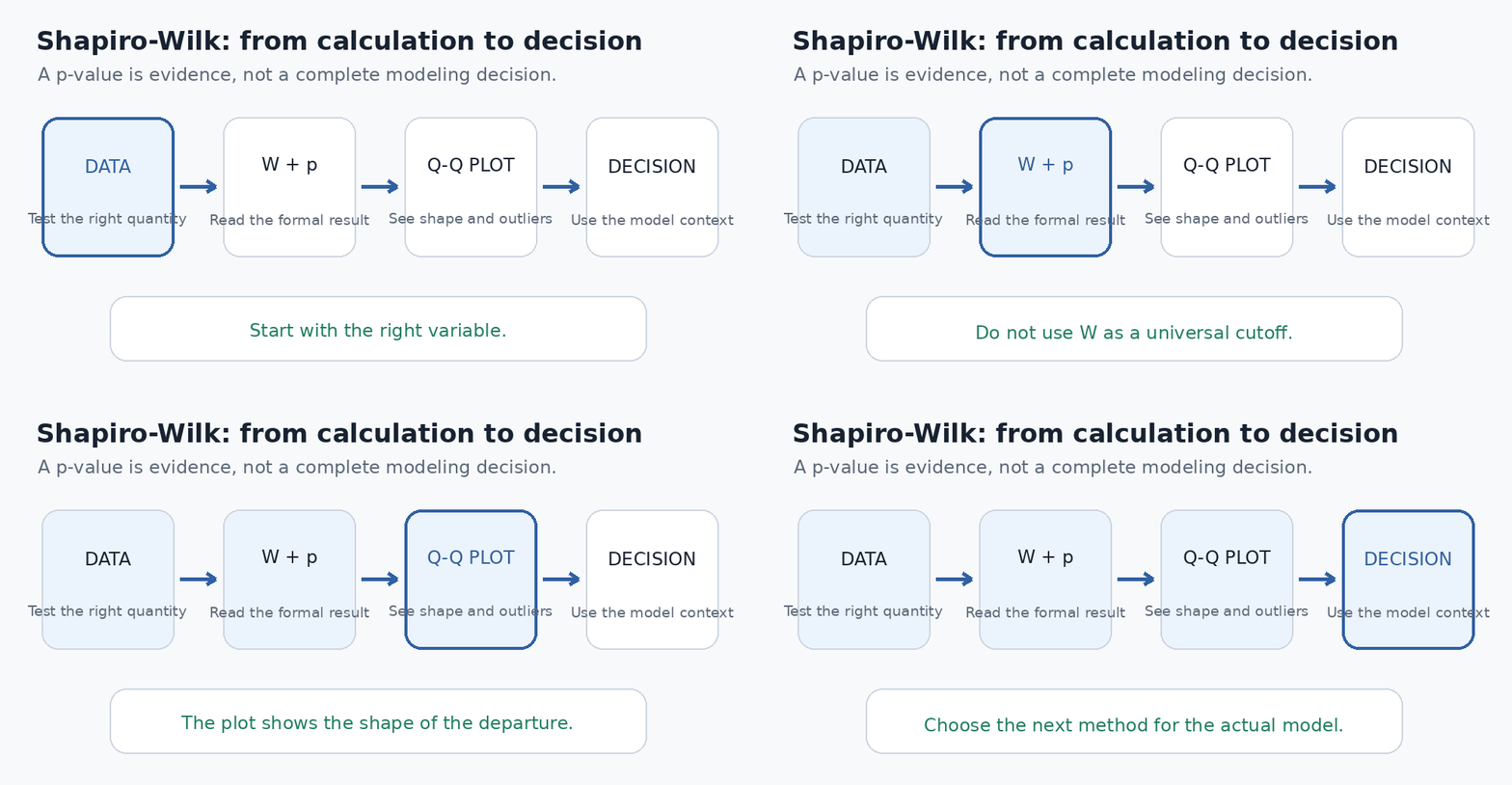
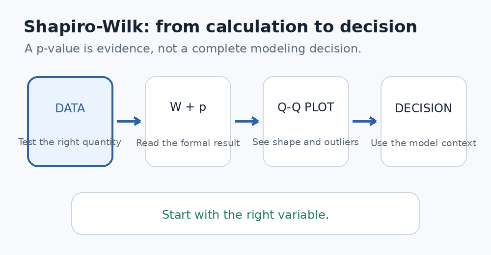
The more important decision comes after the calculation. A Shapiro-Wilk result should be interpreted alongside sample size, a Q-Q plot, outliers or ties, and the assumptions of the analysis you actually plan to run. In regression and ANOVA, for example, the relevant normality assumption generally concerns model errors or residuals, not whether the raw outcome variable itself forms a bell curve. [5]
What Is the Shapiro-Wilk Test?
The Shapiro-Wilk test is a formal test of compatibility with a normal, or Gaussian, population distribution. Samuel Shapiro and Martin Wilk introduced the method in 1965 in Biometrika. [1] The test examines the ordered sample values and asks how closely their pattern agrees with the order statistics expected from a normal distribution.
Its hypotheses are simple. The null hypothesis, H₀, states that the sample comes from a normally distributed population. The alternative hypothesis, H₁, states that it does not. A small p-value is evidence against H₀; a large p-value is not evidence that H₀ has been proven true.
What do W and the p-value measure?
W summarizes how closely the ordered data agree with the pattern expected under normality. NIST gives the standard statistic as a squared weighted sum of the ordered observations divided by the sample sum of squared deviations from the mean. Small values of W are evidence of departure from normality. [2]
In practice, W usually moves closer to 1 as the sample better matches the expected normal pattern. But W has no universal pass mark. A value such as W = 0.95 can be non-significant in one sample and highly significant in another because the sampling distribution of W depends on n.
Shapiro-Wilk Test Calculator: What to Enter and Check First
Place the interactive calculator near the top of the page so utility-first users can enter data immediately. The calculator should accept numeric observations and return at least the sample size, W statistic, p-value, the chosen significance level, and a cautious interpretation. It should also explain invalid inputs instead of returning a generic error.
The most important pre-calculation check is conceptual: make sure you are testing the quantity that your downstream model assumes to be normal. For a paired t-test, test the paired differences. For regression and ANOVA, inspect model residuals or errors. Testing a pooled raw outcome can create apparent non-normality that simply reflects genuine differences between groups. [5]
How many observations are required?
Current R documentation for shapiro.test() accepts between 3 and 5,000 non-missing observations. Its p-values are exact for n = 3 and otherwise use Royston-based approximations. [3] SciPy also requires at least three observations and notes that for N > 5,000 the W statistic may remain accurate while its p-value may not be. [4] The 5,000 boundary is therefore an implementation caution, not a scientific law that makes observation 5,001 unusable.
Also check for missing values, zero variance, non-numeric entries, and heavy rounding. If every observation is identical, there is no meaningful continuous-distribution shape to assess. If the data contain many ties because of rounding or coarse measurement, interpretation requires caution because Shapiro-Wilk is sensitive to grouping and ties. [6]
How to Interpret Shapiro-Wilk Test Results
| Result | Formal decision at α = .05 | What you can say |
|---|---|---|
| p < .05 | Reject H₀ | The sample provides statistically significant evidence against a normal population model. |
| p ≥ .05 | Fail to reject H₀ | The sample does not provide sufficient evidence against normality; this is not proof of normality. |
| W close to 1 | No decision by itself | The ordered observations agree relatively closely with the normal-order pattern. |
| Lower W | No universal cutoff | The sample shows greater departure from the expected normal pattern; significance still depends on n. |
How to interpret p < 0.05
At α = .05, p < .05 means you reject the null hypothesis of normality. That is a statement about evidence against an exact normal population model. It is not a command to abandon every parametric method. The practical question is whether the detected departure is severe enough, and of the right kind, to threaten the inference you want to make.
How to interpret p ≥ 0.05
A non-significant result means you failed to detect convincing evidence against normality. It does not establish that the population is exactly normal. This distinction matters most in small samples, where a test can have limited ability to detect skewness, tail problems, or multimodality.
Why W can be close to 1 and still significant
With large n, even a small systematic departure can become statistically detectable. For example, a mildly skewed sample can produce a W value very close to 1 yet a very small p-value when thousands of observations are available. Statistical detectability and practical importance are different questions.
Four Common Result Patterns and What to Do Next
| Pattern | Interpretation | Next step |
|---|---|---|
| p ≥ .05; Q-Q plot broadly straight | No strong evidence against normality | Proceed if the other assumptions of the intended analysis are reasonable. |
| p < .05; clear skew or outlier pattern | The departure is both statistical and visually interpretable | Investigate the cause and consider a suitable model, robust method, transformation, or non-parametric alternative. |
| p < .05; very large n; only mild Q-Q deviation | A small departure is statistically detectable | Evaluate whether the planned method is sensitive to that departure before changing analyses. |
| p ≥ .05; very small n; suspicious Q-Q plot | The test may have limited power | Do not claim normality; use the graph, study design, and model sensitivity to guide the decision. |
This four-pattern framework is more useful than a binary “normal/not normal” badge because it connects the formal test to the actual analytical decision.
Why You Should Pair Shapiro-Wilk With a Q-Q Plot
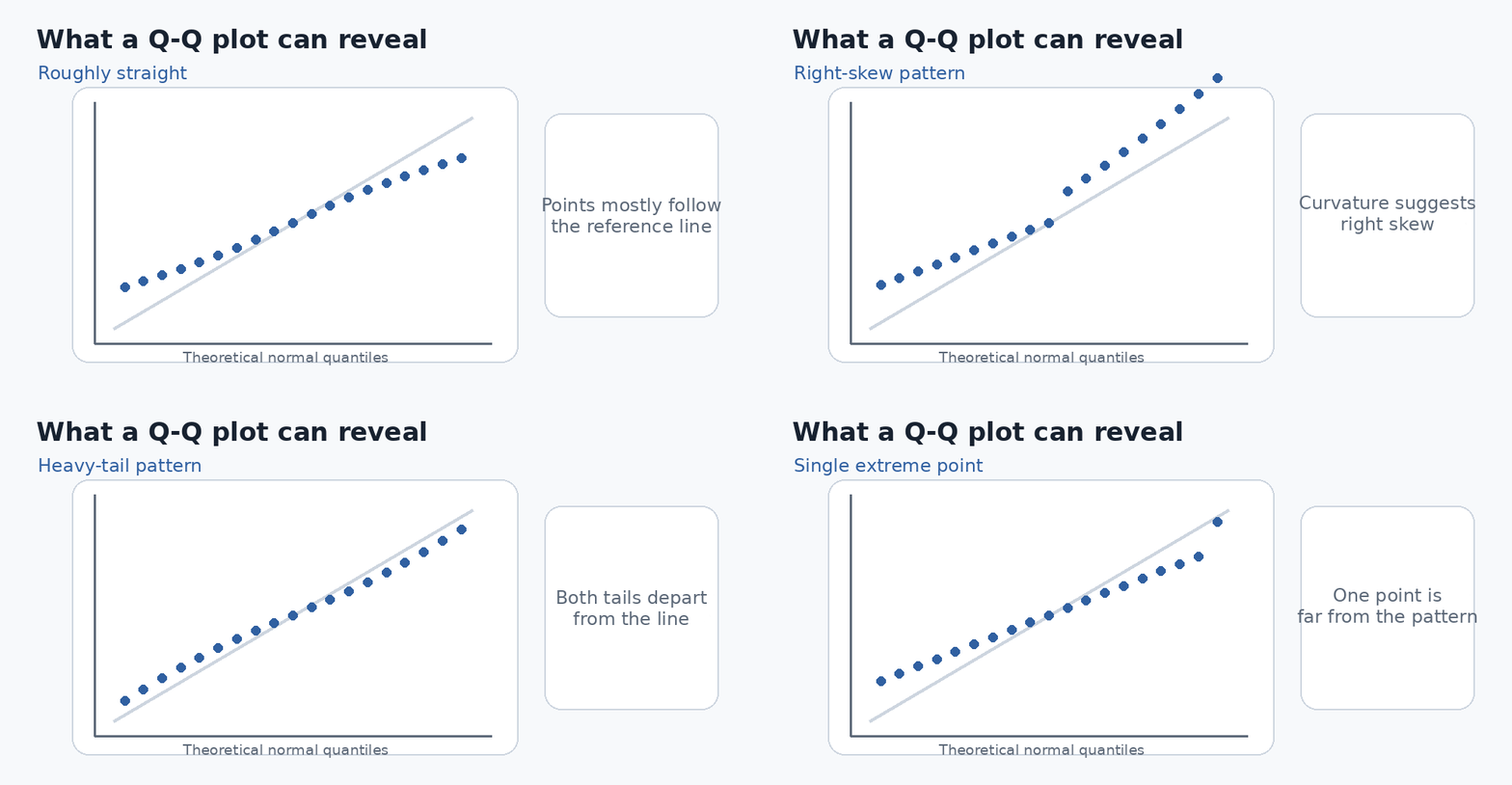
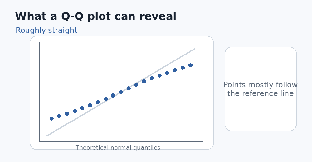
A Shapiro-Wilk p-value tells you whether there is detectable evidence against normality. A Q-Q plot helps explain how the sample departs from normality. Points that track the reference line support a broadly compatible shape; systematic curvature can indicate skewness; both tails bending away can indicate heavier or lighter tails; and one isolated point can reveal an influential outlier.
A histogram can add context for multimodality, gaps, floor or ceiling effects, and obvious data-entry problems. However, histogram appearance depends on bin choice, so it is better used as a companion diagnostic than as a pass/fail rule.
What Actually Needs to Be Normal?
This is the most important distinction for avoiding misuse. “My data are not normal” is often too vague to be statistically useful. The relevant quantity depends on the model.
| Planned analysis | Normality question to assess |
|---|---|
| One-sample t-test | For exact small-sample inference, consider the distribution of observations around the hypothesized mean, especially skewness and extreme tails. |
| Paired t-test | Assess the distribution of the within-pair differences, not the two raw columns separately. |
| Independent t-test | Consider the error/distribution structure within groups. Do not test a pooled mixture of groups with different means. |
| ANOVA | Assess the fitted model errors or residuals in the context of the design. |
| Linear regression | Assess errors or residuals when normality is relevant to the intended inference; the predictors and outcome do not each need a normal marginal distribution. |
| Pearson correlation | A Shapiro test on each variable alone does not establish the joint distributional assumptions used for exact inference. |
A 2025 study of regression workflows documented widespread testing of raw data instead of residuals and argued for greater emphasis on model diagnostics rather than mechanical normality pretesting. [5] That is a useful corrective to the common workflow “test the raw column, then choose parametric or non-parametric.”
Sample Size Changes What the Test Can Tell You
Small samples
With a small sample, failure to reject H₀ provides only limited reassurance. A visibly skewed population can still produce a small random sample that looks unremarkable. In this setting, graphical diagnostics, knowledge of the measurement process, and the sensitivity of the planned analysis deserve more weight.
Moderate samples
This is often where Shapiro-Wilk is most intuitively useful: there can be enough information to detect meaningful departures while Q-Q plots remain easy to interpret. The test still should not replace visual and model-based diagnostics.
Large samples
With hundreds or thousands of observations, increasingly small departures become detectable. The useful question shifts from “is the population exactly normal?” to “does the observed departure matter for the analysis?” SciPy adds a separate computational caution above N = 5,000 because its p-value may not be accurate in that range. [4]
Limitations and Common Mistakes
Treating p ≥ .05 as proof of normality
This confuses failure to reject with confirmation. A large p-value means the sample did not provide strong evidence against H₀; it does not calculate the probability that H₀ is true.
Automatically switching to a non-parametric test after p < .05
The conventional rule is understandable but incomplete. A significant Shapiro-Wilk test shows evidence against exact normality; it does not independently show that a t-test, ANOVA, or regression analysis is invalid. Robustness depends on sample size, group balance, skewness, tail behavior, unequal variances, and influential observations. Recent simulation work on regression workflows found relatively small performance differences across several common decision strategies and emphasized correct residual diagnostics. [5]
Using a universal W cutoff
Rules such as “W > .95 is normal” are not defensible as general thresholds. W must be interpreted through its sample-size-dependent reference distribution and p-value, then considered in context.
Ignoring ties, rounding, and coarse discrete scales
Royston showed that the statistic can be sensitive to ties produced by grouping or rounding. [6] A single 1-to-5 Likert item, for example, has only five possible values and many ties, so asking whether it follows a continuous normal distribution is usually less informative than choosing a model appropriate to the ordinal measurement process.
Deleting an outlier just to make p non-significant
An extreme observation should be investigated, not erased because it changes the normality result. Correct genuine recording errors. If the value is real, determine whether it represents a different process, an influential but valid observation, or a feature that calls for a robust method or different model.
What to Do If the Data or Residuals Are Not Normal
Start with diagnosis rather than transformation. Inspect the Q-Q plot, raw observations, group structure, and residuals. Look for data errors, subgroups, floor or ceiling effects, influential observations, and structural skewness. Then ask whether normality is truly required for the inference you plan to make.
If the model is sensitive to the departure, several responses may be reasonable. A transformation such as log, square-root, Box-Cox, or Yeo-Johnson can sometimes improve a model, but it also changes the scale and interpretation of effects. A robust estimator, bootstrap or permutation approach, a generalized model built for the observed distribution, or a non-parametric procedure may be more suitable. The choice should follow the research question and data-generating process, not the goal of forcing p above .05.
Mann-Whitney U and Kruskal-Wallis are useful alternatives in appropriate settings, but “non-parametric” does not mean “assumption-free,” and these methods do not always test the same estimand as a mean-based parametric procedure. Treat them as different analytical tools, not automatic replacements.
Shapiro-Wilk Compared With Other Normality Tests
Shapiro-Wilk vs Kolmogorov-Smirnov
Shapiro-Wilk is specifically designed for normality. The classical Kolmogorov-Smirnov test compares an empirical distribution with a fully specified reference distribution. If normal parameters are estimated from the same sample, the ordinary K-S critical values are not directly interchangeable; a modification such as Lilliefors is used. For a normality-specific formal test, Shapiro-Wilk is usually the more natural default.
Shapiro-Wilk vs Anderson-Darling
Anderson-Darling is another goodness-of-fit approach and gives extra weight to the distribution tails. NIST highlights this tail weighting as an important distinction from the K-S statistic. [2] If tail behavior is especially important, Anderson-Darling can provide a useful complementary perspective.
Shapiro-Wilk vs D’Agostino-Pearson
D’Agostino-Pearson combines departures in skewness and kurtosis into an omnibus statistic, while Shapiro-Wilk evaluates the broader ordered-sample pattern. Different tests emphasize different features, so disagreement is possible. The right response to disagreement is to inspect the distribution and understand what each test is detecting rather than choosing whichever p-value supports a preferred conclusion.
How to Run Shapiro-Wilk in SPSS, R, Python, and Excel
SPSS
In IBM SPSS Statistics, the familiar Explore workflow is Analyze → Descriptive Statistics → Explore, then Plots → Normality plots with tests. IBM’s documentation also recommends requesting the normality plots in that workflow. [7] In output, “Sig.” is the p-value.
R
In R, use shapiro.test(x). The current documentation accepts 3 to 5,000 non-missing values and returns W plus an approximate p-value, with an exact p-value only for n = 3. [3]
Python / SciPy
In Python, scipy.stats.shapiro(x) returns the statistic and p-value. SciPy also provides explicit NaN-handling options and warns about p-value accuracy above N = 5,000. [4]
Excel
Microsoft’s current Excel function list does not include a native SHAPIRO or SHAPIRO.WILK worksheet function. [8] Excel implementations therefore depend on a custom formula, add-in, script, or external calculator. For reproducible research, a documented statistical package is usually easier to audit than an undocumented spreadsheet implementation.
How to Report a Shapiro-Wilk Test
Report the W statistic, p-value, the sample or residuals tested, and enough context to show what assumption was evaluated. If α was specified in advance, include it when useful.
For a non-significant result, a cautious example is: “The Shapiro-Wilk test did not show a statistically significant departure from normality, W = 0.975, p = .957.” For a significant result: “The Shapiro-Wilk test indicated evidence of departure from normality, W = 0.696, p < .001.”
If the result changed the analysis, report that reasoning too. For example, explain that residual diagnostics showed strong right skew and influential observations, leading to a different model. Avoid the unsupported statement “the normality assumption was met” when you only tested a raw variable.
Frequently Asked Questions
What is a good Shapiro-Wilk p-value?
There is no universally “good” p-value. At α = .05, p ≥ .05 means you fail to reject normality; p < .05 means there is evidence against it. The p-value should not be treated as a score of how normal the sample is.
What does W = 0.95 mean?
It means the sample has fairly high agreement with the expected normal-order pattern, but 0.95 is not a universal pass threshold. The same W can have different statistical meaning at different sample sizes.
Can I use a t-test if Shapiro-Wilk is significant?
Possibly. A significant normality test does not automatically invalidate a t-test. The decision depends on the kind of t-test, n, balance, variance structure, degree of skewness, tail behavior, outliers, and what inferential target matters. Severe departures in small samples deserve more concern than tiny detectable departures in large, balanced samples.
Should I test raw data or residuals?
For regression and ANOVA, assess the model errors or residuals when normality is relevant to the inference. For a paired t-test, assess paired differences. Testing raw columns without identifying the actual model assumption is a common mistake. [5]
Can I use Shapiro-Wilk for Likert data?
For a single coarse Likert item, the many ties and ordinal scale make a continuous normality test difficult to interpret. A multi-item composite with many possible values is a different case, but the choice should still follow the model and measurement scale rather than a mechanical p-value rule.
What if the Q-Q plot looks normal but Shapiro-Wilk is significant?
Check sample size and where the Q-Q plot departs from the line. With large n, a subtle but systematic tail or curvature pattern can be statistically significant. Decide whether that feature is consequential for your intended analysis rather than ignoring either diagnostic.
Is Shapiro-Wilk better than Kolmogorov-Smirnov?
For the specific task of normality testing, Shapiro-Wilk is usually a more appropriate default than mechanically applying the classical K-S test. But no formal test is a substitute for understanding the model, sample size, and distribution shape.
What if I have more than 5,000 observations?
Do not interpret 5,000 as a universal scientific cutoff. It is a documented limit for R’s shapiro.test() and a p-value accuracy warning in SciPy. [3] [4] With very large datasets, graphical diagnostics, residual behavior, effect sizes, and model robustness usually provide more decision value than testing for microscopic departures from exact normality.
Quick Summary: Use the Result as Evidence, Not a Gatekeeper
A Shapiro-Wilk test calculator is most useful when it helps you move from calculation to diagnosis and then to a model decision. If p ≥ .05, say that you did not find sufficient evidence against normality, not that normality was proven. If p < .05, identify the shape and source of the departure before changing methods.
The highest-impact practical step is to test the right quantity. For paired analyses, that may be the differences; for regression and ANOVA, it is generally the error or residual structure. Then combine W, the p-value, sample size, the Q-Q plot, outliers or ties, and the sensitivity of the intended analysis. That gives the Shapiro-Wilk test calculator and interpretation process its real value: not a green or red badge, but a defensible next decision.
Sources and Verification
[2] NIST/SEMATECH e-Handbook: Anderson-Darling and Shapiro-Wilk tests.
[4] SciPy documentation: scipy.stats.shapiro, including the N > 5,000 p-value caution.
[7] IBM SPSS Statistics 31 documentation: Explore workflow and normality plots with tests.
[8] Microsoft Excel functions reference. No native SHAPIRO worksheet function is listed.
[9] Google Search Central: optimization guidance for generative AI features in Search.
[10] Google Search Central documentation updates, including the 2026 FAQ rich-result deprecation.
Try it in DataClue
Ready to run Shapiro-Wilk Test?
Test whether a sample comes from a normally distributed population.
Run Shapiro-Wilk Test