
Simple Linear Regression: Beginner Guide to the Model and Scatter Plots
Learn simple linear regression step by step. Understand dependent and independent variables, scatter plots, regressand and regressor, slope, intercept
Simple Linear Regression: A Beginner Guide to Regression and the Model
Simple linear regression is a way to study how one variable changes with another variable. This lesson focuses on meaning, variables, scatter plots, the regression model, and basic assumptions before any lengthy calculation begins.
In this lesson
- What regression means
- Dependent Y and independent X
- Deterministic and probabilistic relationships
- Scatter diagrams
- Activity
- The simple linear regression model
- Intercept, slope, and random error
- Basic assumptions
1. What Is Regression?
The word regression has an important place in the history of statistics. The source text connects the idea with Francis Galton and his work on the heights of children and parents. He noticed a tendency for extreme values to move toward an average across generations.
Modern regression has a wider meaning. Regression analysis studies dependence. We choose a variable that we want to explain or predict. That variable is Y. We then choose a variable that may help explain Y. That variable is X.
Dependence does not mean that X is the only cause of Y. A regression can describe a useful relationship even when many other factors affect Y. That is one reason the random error term matters.
Regression vocabulary
| Symbol | Main term | Plain meaning | Other textbook names |
|---|---|---|---|
| Y | Dependent variable | The variable we want to explain or predict | Regressand, predictand, response variable, explained variable |
| X | Independent variable | The variable used to explain or predict Y | Regressor, predictor, regression variable, explanatory variable |
| α | Intercept | Expected Y when X equals zero | Constant term |
| β | Slope | Expected change in Y for a one unit increase in X | Regression coefficient |
| εᵢ | Random error | Other influences on Y that are not included in X | Random deviation, error component |
2. Dependent Variable Y and Independent Variable X
The dependent variable Y is the outcome we want to explain or predict. The independent variable X is the variable used to explain or predict Y. In a scatter diagram, X is usually placed on the horizontal axis and Y on the vertical axis.
| Role | Y, dependent variable | X, independent variable |
|---|---|---|
| Main question | What are we trying to explain? | What may help explain it? |
| Graph axis | Vertical axis | Horizontal axis |
| Example, study and marks | Exam marks | Study hours |
| Example, advertising and sales | Sales | Advertising spending |
A useful question is simple. What am I trying to explain? The answer usually belongs in Y. Then ask what variable may help explain it. That variable usually belongs in X.
3. Deterministic and Probabilistic Relationships
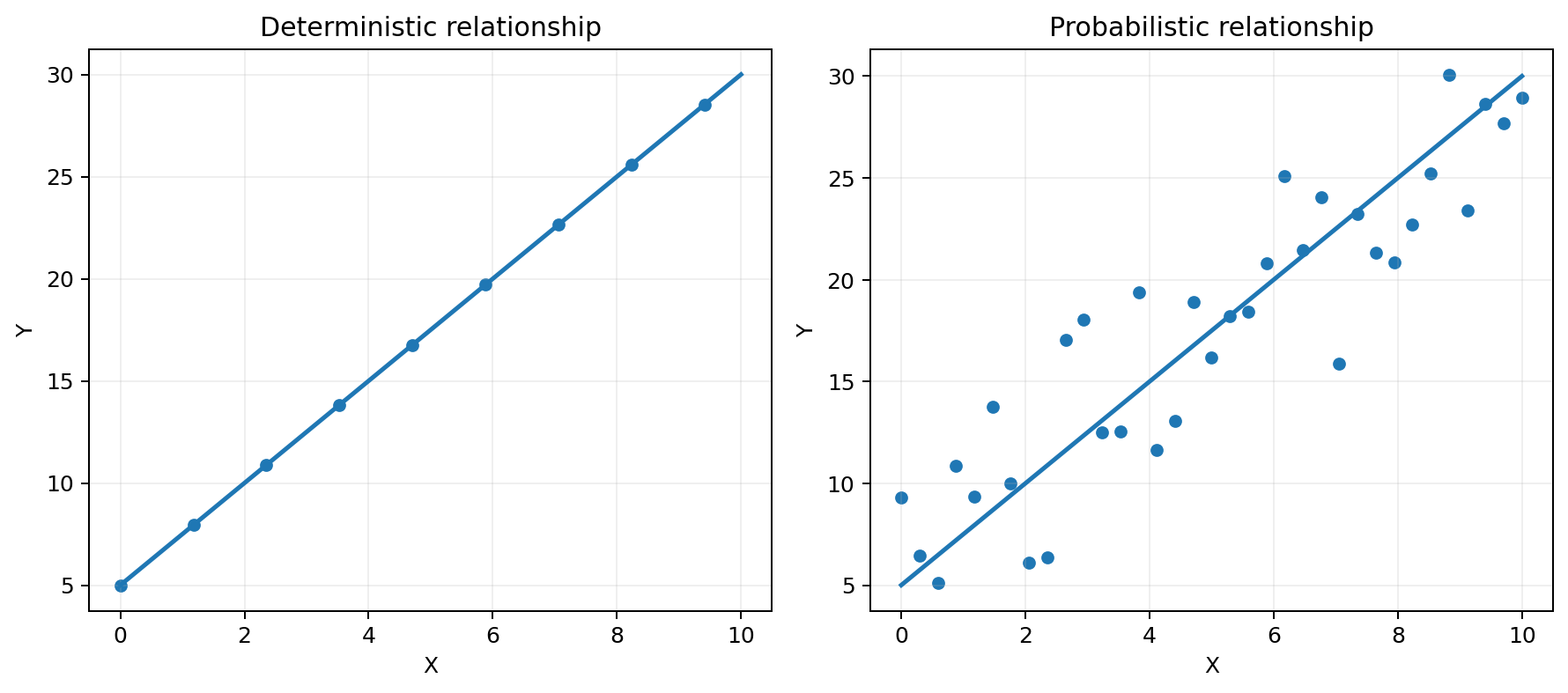
A deterministic relationship is exact. Once X is known, Y is fixed by the rule. A probabilistic relationship is different. X helps explain Y, but the same X value can still be linked with different Y values because other influences are present.
| Feature | Deterministic relationship | Probabilistic relationship |
|---|---|---|
| Meaning | Knowing X fixes Y exactly | Knowing X helps, but Y can still vary |
| Need for random error | No random error is needed in the exact rule | A random error term is needed |
| Simple example | Y = 5 + 2X as an exact rule | Marks related to study hours, with other influences |
| Scatter pattern | Points lie exactly on the rule | Points vary around an expected pattern |
4. Scatter Diagrams Come Before the Equation
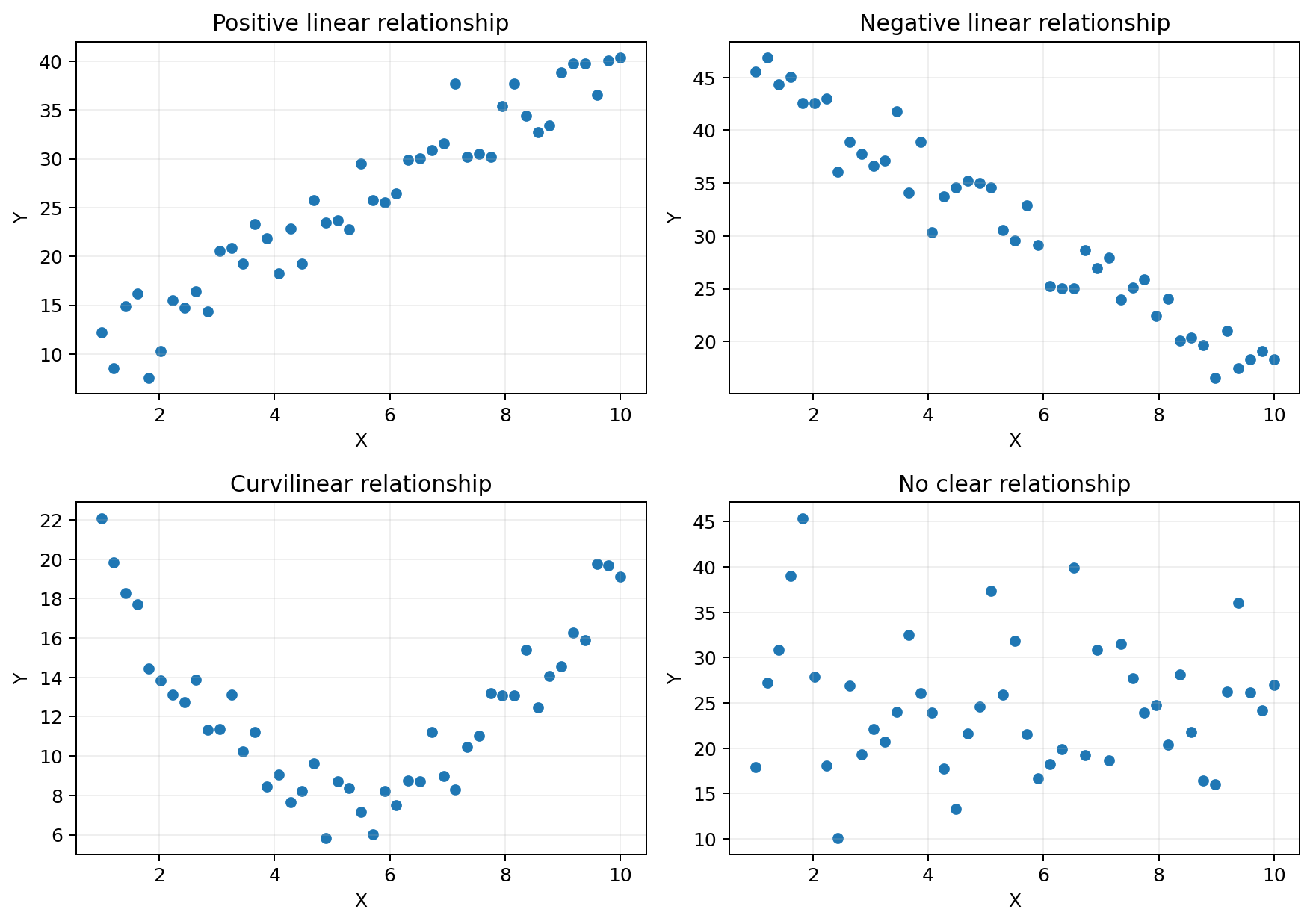
A scatter diagram plots paired observations. Each point represents one X value and one Y value. Before fitting any line, look at the shape of the point cloud.
Animated scatter pattern explorer
Choose a pattern. Watch the points appear, then name the relationship before reading the label.
| Pattern | What the points look like | What it suggests for a straight line | Simple example |
|---|---|---|---|
| Positive linear | Points rise as X increases | β is expected to be positive | Study hours and marks |
| Negative linear | Points fall as X increases | β is expected to be negative | Price and quantity demanded in a simple example |
| Curvilinear | Points follow a curve | A straight line may not describe the pattern well | A response that rises and then levels or bends |
| No clear relationship | Points form a cloud without direction | A useful linear slope may be near zero | Two variables with no clear pattern |
How to read the patterns
Positive linear relationship. The point cloud rises from left to right. Larger X values tend to be linked with larger Y values.
Negative linear relationship. The point cloud falls from left to right. Larger X values tend to be linked with smaller Y values.
Curvilinear relationship. The points follow a bend or curve. A straight line may miss an important part of the pattern.
No clear relationship. The points form a cloud with no strong upward, downward, or curved direction.
5. Activity: Identify X, Y, and Direction
Try each situation before reading the answer table. First identify the outcome you want to explain. Then identify the possible predictor. Finally, decide the expected direction.
| Situation | Suggested X | Suggested Y | Expected direction | Other factors that can affect Y |
|---|---|---|---|---|
| Study hours and exam marks | Study hours | Exam marks | Positive | More study time may be linked with higher marks, but sleep, prior knowledge, and test difficulty also matter. |
| Advertising and sales | Advertising spending | Sales | Positive | More advertising may be linked with higher sales, but price, season, and competition also matter. |
| Income and expenditure | Household income | Household expenditure | Usually positive | Higher income may be linked with higher spending, but saving habits and household size also matter. |
| Height and weight | Height | Weight | Usually positive | Taller people may tend to weigh more, but body type, age, and other factors also matter. |
The final column shows why a simple regression is usually probabilistic. Even when X is useful, it is rarely the only influence on Y.
6. The Simple Linear Regression Model
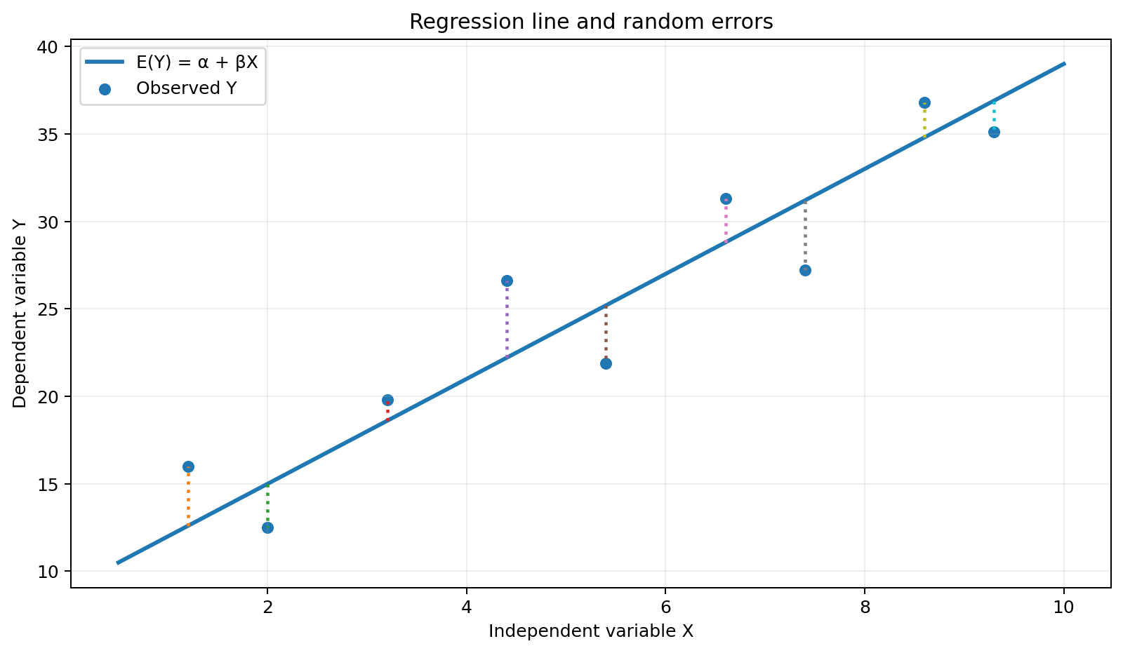
This equation separates the observed value of Y into two parts. The first part, α + βXᵢ, is the systematic linear relationship. The second part, εᵢ, is the random deviation from that relationship.
| Symbol | Name | Meaning |
|---|---|---|
| Yᵢ | Observed dependent variable | The actual Y value for observation i |
| Xᵢ | Observed or fixed independent variable | The X value for observation i |
| α | Intercept | Expected Y when X equals zero |
| β | Slope or regression coefficient | Expected change in Y when X rises by one unit |
| εᵢ | Random error | Difference caused by influences not represented by X |
7. Intercept α, Slope β, and Random Error εᵢ
What does α mean?
The intercept α is the expected value of Y when X equals zero. On a graph, it is where the expected regression line meets the Y axis. This interpretation is useful only when X equals zero makes sense in the real problem.
What does β mean?
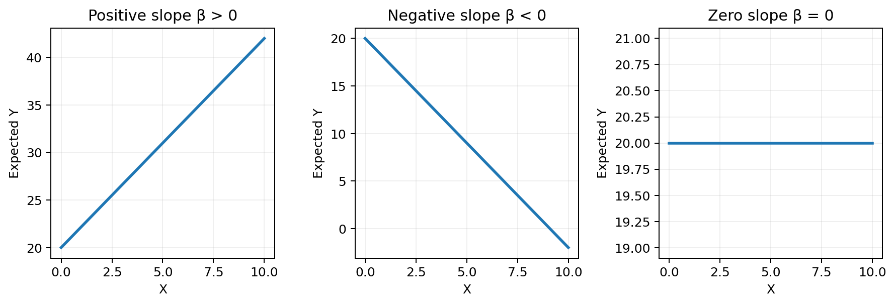
The slope β is the regression coefficient. It tells us the expected change in Y when X increases by one unit. A positive β makes the expected line rise. A negative β makes it fall. A zero β makes it flat.
What does εᵢ mean?
The random error εᵢ captures the part of Y that the simple X variable does not explain. It can reflect omitted influences, natural variation, and other differences among observations. It is not limited to a data entry mistake.
8. The Expected Regression Line
The source assumes that E(εᵢ) = 0. This means positive and negative errors balance out on average. For a given X, the expected value of Y is therefore α + βX.
9. Basic Assumptions of the Simple Linear Regression Model
These assumptions describe the introductory model in the source. At this stage, the goal is understanding. Formal testing and advanced diagnostics belong to later lessons.
| Assumption | Formula | Plain English meaning | What to remember |
|---|---|---|---|
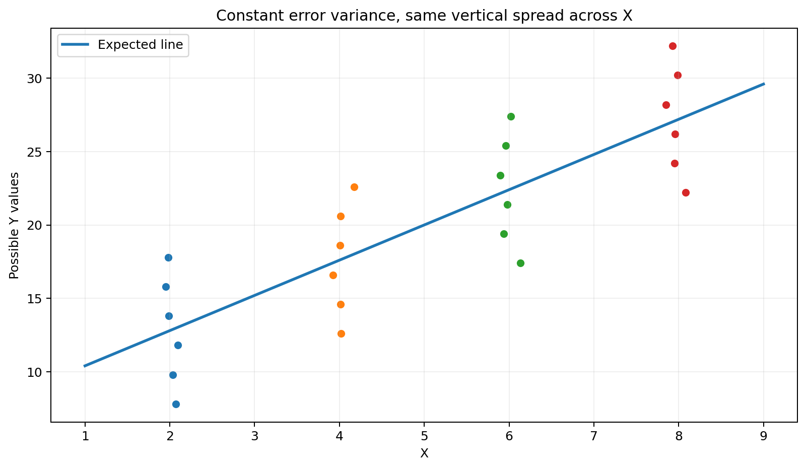
| Mean error is zero | E(εᵢ) = 0 | Positive and negative errors balance out on average. | The expected regression line is E(Yᵢ) = α + βXᵢ. |
| Constant error variance | Var(εᵢ) = σ² | The vertical spread of errors is assumed to stay the same for all X values. | This is the homoscedasticity assumption. |
| Errors are unrelated across observations | E(εᵢεⱼ) = 0 for i ≠ j | The error for one observation does not systematically move with the error for another. | The errors are treated as independent across observations in the textbook model. |
| X is independent of the error | E(Xᵢεᵢ) = 0 | X should not move together with the omitted random part of Y. | The explanatory variable is separated from the error term. |
| Normal error distribution | εᵢ is Normal with mean 0 and variance σ² | The textbook assumes a normal shape for the error distribution. | For a given X, Y is then normal around α + βX. |
10. Mini Interpretation Examples
Study hours and marks. If β is positive, one more hour of study is linked with a higher expected mark. The exact mark can still vary because ε includes other influences.
Advertising and sales. If β is positive, more advertising is linked with higher expected sales. A large ε could reflect price changes, competitor actions, or seasonal demand.
Income and expenditure. If β is positive, higher income is linked with higher expected expenditure. Household size and saving preferences can enter the error term.
Height and weight. If β is positive, greater height is linked with higher expected weight. The relationship is not exact because age, body type, and other factors matter.
11. Common Beginner Mistakes
| Mistake | Better way to think about it |
|---|---|
| Switching X and Y without thinking | Choose the roles from the research question. Ask what you want to explain, then place that variable in Y. |
| Thinking positive means perfect | A positive relationship only means the general direction is upward. Points can still be far from a straight line. |
| Thinking every relationship is linear | A scatter plot may show a curve. A straight line can be a poor description of that pattern. |
| Confusing intercept and slope | The intercept is a level at X equals zero. The slope is a change in Y for a one unit change in X. |
| Thinking ε means a typing mistake | The error term represents many influences that are not included in the simple model. It is not limited to data entry errors. |
| Thinking a scatter plot gives the equation | The scatter plot shows shape and direction. It does not by itself calculate α and β. |
12. Summary
| Term | One line meaning |
|---|---|
| Regression | Studies how the expected value of Y depends on X. |
| Y | Dependent variable, the outcome we want to explain. |
| X | Independent variable, the predictor used to explain Y. |
| Scatter diagram | A first visual check of direction and shape. |
| Positive pattern | Y tends to rise as X rises. |
| Negative pattern | Y tends to fall as X rises. |
| Curvilinear pattern | A straight line may not fit the relationship well. |
| No relationship | No clear direction appears in the point cloud. |
| α | Intercept, expected Y when X equals zero. |
| β | Slope, expected change in Y for one unit more X. |
| εᵢ | Random part of Y not represented by X in the simple model. |
Try it in DataClue
Ready to run Simple Linear Regression?
Fit a simple regression model with one numeric predictor (X) and one numeric outcome (Y) using OLS.
Run Simple Linear Regression