
Statistical Power Calculator & Power Analysis Guide
Astatistical power calculatorhelps you determine how many observations you need, how much power a planned sample provides, or the smallest effect your study can reliably detect. Power is the probability that a test will…
Statistical Power Calculator & Power Analysis Guide
A statistical power calculator helps you determine how many observations you need, how much power a planned sample provides, or the smallest effect your study can reliably detect. Power is the probability that a test will reject the null hypothesis when a specified alternative effect is truly present, so the calculation is useful only when its assumptions match the study you actually plan to run.
The practical goal is not to choose familiar defaults and produce the smallest affordable sample. It is to define an effect that matters, match the calculation to the intended analysis, make uncertainty in the assumptions visible, and decide whether the planned study can answer the question that justifies collecting the data.
Statistical Power Calculator: Calculate Sample Size, Power, or Minimum Detectable Effect
Power analysis answers different questions depending on what is already fixed. Before collecting data, an a priori power analysis usually solves for the sample size required to detect a specified effect at a chosen significance level and target power. When the available sample cannot change, a sensitivity analysis can instead solve for the minimum detectable effect. If sample size and effect are both specified, the calculation can estimate the planned power of that design.
| Planning question | Known inputs | Useful output |
|---|---|---|
| How many observations do I need? | Effect, alpha, target power, statistical design | Required sample size |
| What can my available sample detect? | Sample size, alpha, target power, statistical design | Minimum detectable effect |
| How much power does this plan provide? | Sample size, effect, alpha, statistical design | Planned statistical power |
A bare result such as “N = 128” is incomplete. A defensible result says something closer to: “For an equal-allocation, two-sided independent-samples t-test, α = .05, target power = .80, and Cohen's d = .50, the calculated sample is approximately 64 analyzable participants per group.” The assumptions are part of the answer.
What Is Statistical Power and Why Does It Matter?
Statistical power is the probability that a statistical test will correctly reject the null hypothesis when a specified alternative hypothesis is true. The official statsmodels documentation describes power as one minus the probability of a Type II error.
If a study has 80% power for a particular effect, that means repeated studies run under the calculation's assumptions would reject the null hypothesis about 80% of the time when that specified effect is truly present. It does not mean there is an 80% probability that the research hypothesis is correct, and it does not mean every possible effect has an 80% chance of detection.
This distinction is why saying a study is simply “powered” or “underpowered” is incomplete. A design can have high power for a large effect and low power for a smaller effect. Power belongs to a test, effect, sample size, alpha level, and set of assumptions.
Statistical power is not the same as statistical significance
Statistical significance is an outcome of the analysis of observed data relative to a prespecified decision threshold such as α = .05. Power describes how often that analysis would detect a specified effect across repeated samples before the outcome is known. A low-powered study can still produce a significant result, and a well-powered study can produce a nonsignificant result.
High power is not a general trust score
Power does not protect a study against selection bias, confounding, poor measurement, protocol deviations, inappropriate models, selective reporting, or other threats to validity. It answers a narrower question: given this statistical model and a particular true effect, how likely is the planned test to meet its rejection rule?
What Inputs Does a Power Analysis Actually Need?
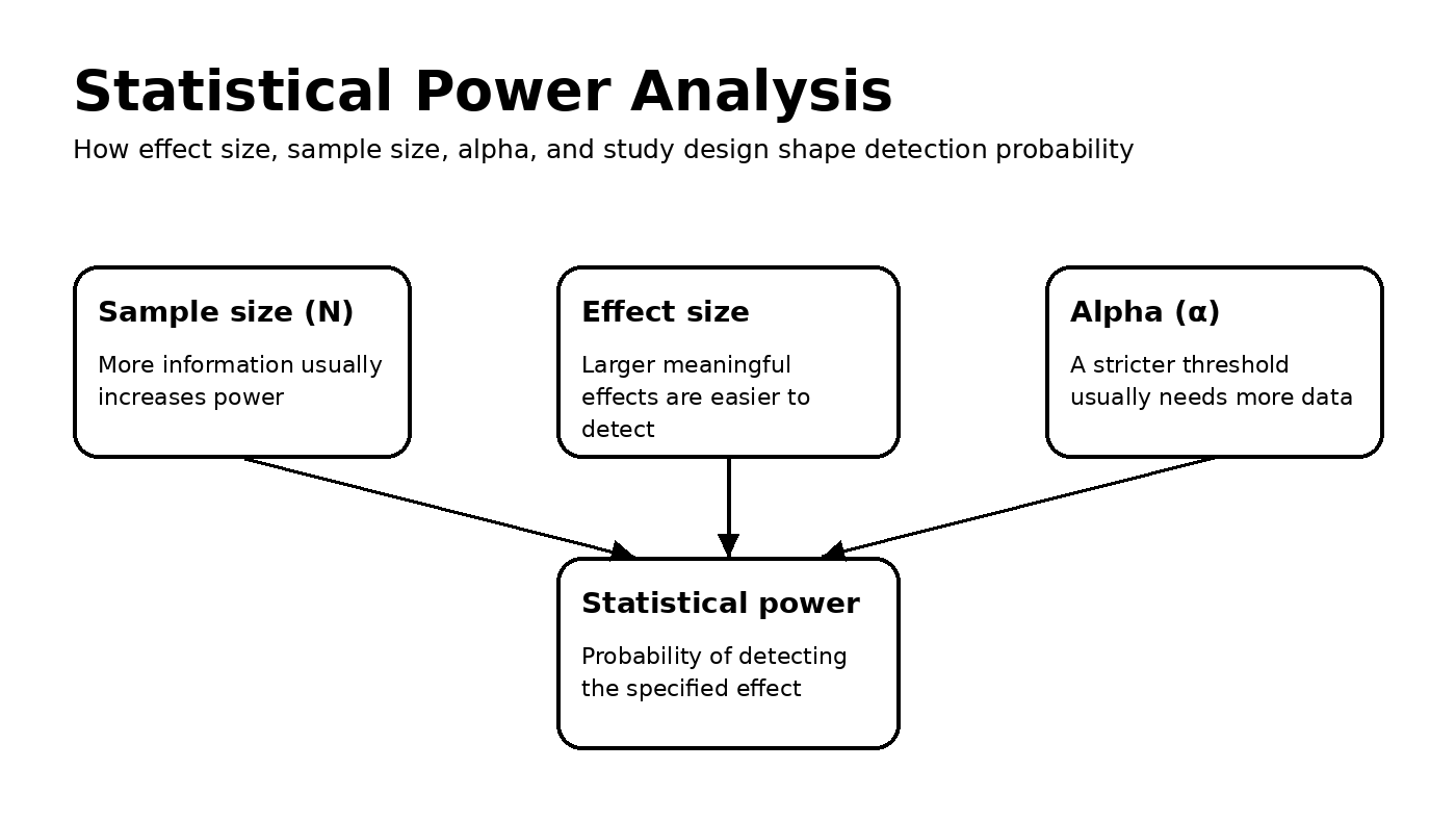
Power is often taught using four connected quantities: sample size, effect size, significance level, and statistical power. That framework is useful, but it is not a universal four-input formula. The actual calculation also depends on the design and statistical test.
| Change | Typical effect, with other assumptions fixed |
|---|---|
| Larger sample size | Power increases |
| Smaller target effect | Required sample size increases |
| Higher target power | Required sample size increases |
| Lower alpha | Required sample size usually increases |
| Greater unexplained variability | Required sample size usually increases |
An independent two-sample t-test may require a standardized mean difference and group allocation ratio. A two-proportion calculation depends on the underlying proportions. A one-way ANOVA needs the number of groups as well as an effect-size definition. Regression calculations depend on the hypothesis being tested and model structure. Repeated measures, cluster randomized trials, survival analyses, and multilevel models require still more design-specific assumptions.
This is reflected in statistical software. G*Power separates procedures across t, F, chi-square, z, and exact-test families, while R's pwr package provides different functions for t-tests, correlations, ANOVA, chi-square tests, general linear models, and proportions.
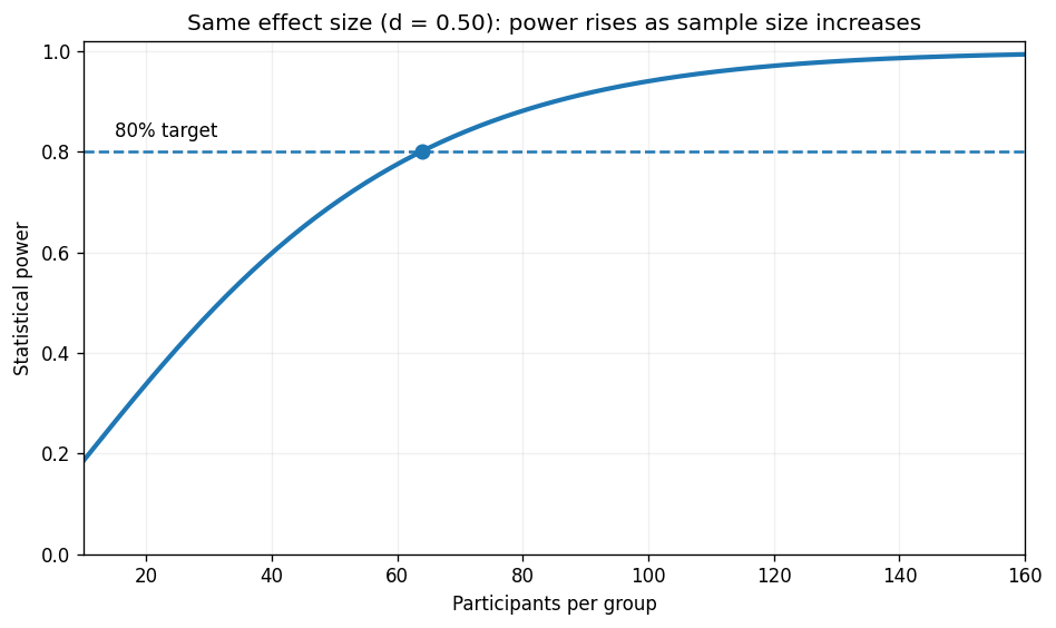
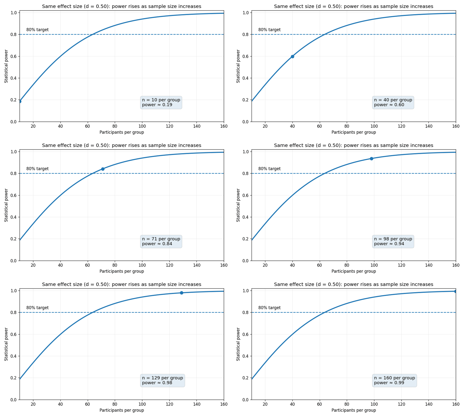
Animated example: Why larger samples increase power
How to Calculate the Sample Size Needed for a Study
Start with the primary outcome and primary hypothesis. The sample-size calculation should match the analysis that will answer that hypothesis, not whichever calculator happens to be easiest to use.
Next, define the smallest effect that would matter. This may be a clinically important difference, an operationally worthwhile lift, a scientifically meaningful correlation, or another decision-relevant threshold. Then estimate any nuisance parameters required by the design, such as a standard deviation, baseline event rate, within-person correlation, allocation ratio, or intracluster correlation.
Choose the significance level and target power, then calculate the required analyzable sample. If the result is fractional, round upward. Only after that should you inflate the recruitment target for expected attrition, exclusions, or unusable measurements.
How to adjust sample size for attrition
Suppose the statistical calculation requires 100 participants with usable final outcomes and you expect 15% attrition. Adding 15% directly gives 115 recruits, but 15% of 115 is 17.25, which leaves fewer than 100 expected completers.
The correct planning relationship is recruitment target = analyzable N ÷ expected retention. With 85% expected retention, 100 ÷ 0.85 = 117.65, so the recruitment target should be rounded up to 118.
Attrition is not the only real-world adjustment. Formal protocols may also need to account for nonadherence, crossover, missing outcomes, clustering, unequal allocation, multiplicity, or other features that change the effective information available for the primary analysis. In clinical research, requirements for documenting those assumptions vary by regulator, funder, institution, field, and study design; the FDA's ICH E9 statistical principles guidance is one example of formal statistical-design guidance rather than a universal rule for all research.
How to Choose an Effect Size Without Fooling Yourself
For many studies, choosing the effect size is more consequential than operating the calculator. A mathematically correct calculation can still produce a poor study if the assumed effect is unrealistically large.
A practical hierarchy is to begin with the smallest real-world difference that would change a decision, then use strong prior studies or historical data to estimate plausible variability and baseline conditions. Pilot data can be useful for feasibility and some nuisance parameters, but a small pilot's observed treatment effect is often too unstable to treat as the definitive effect for the larger study.
A 2025 BMJ tutorial on pilot-trial sample sizes emphasizes that small pilot trials produce imprecise effect estimates and recommends basing definitive-trial effect assumptions on clinically important differences informed by prior evidence and expert knowledge rather than relying mechanically on the pilot's point estimate.
A realistic sensitivity example
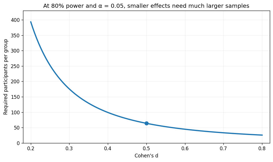
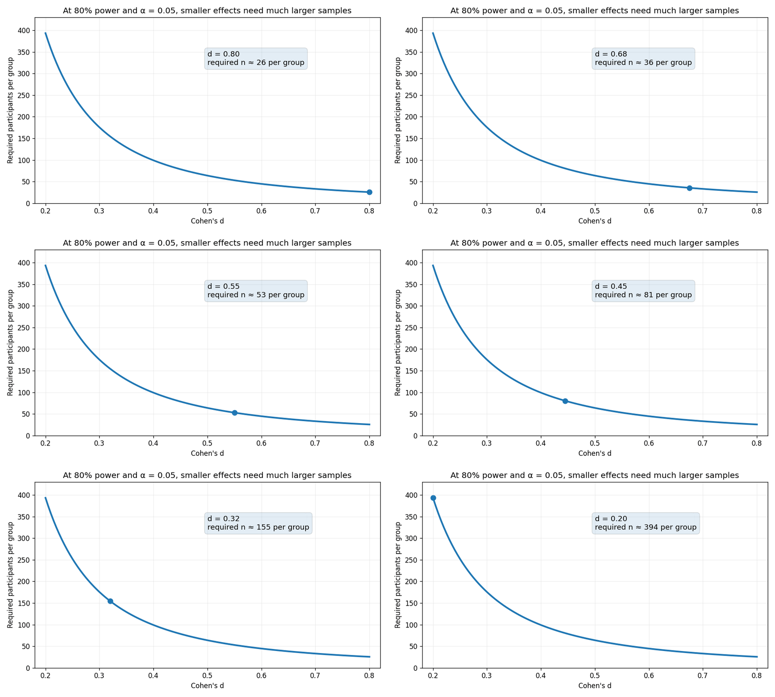
Imagine researchers expect an intervention to improve a score by 5 points, previous evidence suggests a standard deviation of 12, and a 3-point improvement is the smallest difference that would change practice. For a two-sided equal-allocation t-test with α = .05 and 80% power, the optimistic 5-point assumption corresponds to d ≈ .42 and requires about 92 participants per group. Powering for the 3-point meaningful threshold gives d = .25 and requires about 253 per group.
Neither number is automatically “correct.” The important insight is that the study-design decision changes dramatically depending on which effect the study promises to detect. Reporting both scenarios exposes the uncertainty instead of hiding it inside one optimistic assumption.
Animated example: Why small effects require much larger samples
Where Cohen's conventions fit
Cohen's familiar standardized benchmarks are useful as reference points. For d, values around .20, .50, and .80 are traditionally described as small, medium, and large. R's pwr documentation explicitly implements Cohen-style effect-size conventions across several common tests.
Those labels should be a fallback, not a substitute for subject-matter judgment. A statistically “small” effect can be important when an intervention is inexpensive, safe, and applied at scale. A larger standardized effect can still be unimportant if it does not change a real decision.
How Much Statistical Power Should You Use?
There is no universal target that every study must use. Eighty percent is a common convention, while 90% or higher may be reasonable when missing a meaningful effect would have more serious consequences. The target should be justified in the context of the decision, design, feasibility, and any applicable professional or regulatory requirements.
| Target power | Approximate n per group | Approximate total N |
|---|---|---|
| 80% | 64 | 128 |
| 90% | 86 | 172 |
| 95% | 105 | 210 |
These illustrative values use an equal-allocation, two-sided independent-samples t-test with Cohen's d = .50 and α = .05, calculated using the same parameterization documented by statsmodels.stats.power.TTestIndPower. Moving from 80% to 90% power increases the required sample by roughly one-third in this example.
Higher power therefore has a real cost. The most defensible target balances the consequences of a false negative against recruitment burden, time, money, participant exposure, and the value of detecting progressively smaller effects.
A Priori, Sensitivity, and Post Hoc Power Analysis
A priori power analysis
Use an a priori analysis before data collection when you need to determine a sample size for a specified effect, alpha level, desired power, and study design. This is the standard use of power analysis for confirmatory planning.
Sensitivity analysis and minimum detectable effect
Use sensitivity analysis when sample size is constrained by budget, recruitment, rare populations, traffic, or logistics. Instead of pretending the ideal N is feasible, calculate the smallest effect the available sample can detect at the chosen power and alpha. Then decide whether a study that can only detect effects that large would still be useful.
Observed post hoc power
A different practice is to take the effect observed in a completed study, calculate “achieved” or observed power from it, and use that number to interpret the study's p-value. Methodological literature strongly discourages this. A peer-reviewed commentary, “Post hoc Power is Not Informative”, explains why observed post hoc power largely recycles information already present in the statistical result and can be misleading for interpretation.
After a study is complete, the estimated effect and its confidence interval are usually more useful for showing what effect sizes remain compatible with the data. A post-study sensitivity calculation can still answer a design question if the effect being evaluated is specified independently of the observed estimate, but that is different from using observed power to rescue or explain a nonsignificant result.
Power Analysis by Statistical Test and Real-World Use Case
| Design or question | Typical effect/input | Important extra assumption |
|---|---|---|
| Independent two-group means | Raw mean difference + SD, or Cohen's d | Allocation ratio and variance model |
| Paired or pre/post means | Mean change or standardized paired effect | Within-person correlation / SD of differences |
| Correlation | Minimum correlation of interest | Test direction and distribution assumptions |
| One-way ANOVA | Cohen's f or group means/variance | Number of groups and balance |
| Multiple regression | R² change, f², or tested coefficient effect | Number and structure of predictors |
| Two proportions / A-B test | Baseline and target proportions | Allocation, absolute vs relative lift |
| Cluster randomized design | Outcome effect | Cluster size and intracluster correlation |
| Survival analysis | Hazard ratio or survival difference | Expected event count, censoring, accrual |
For straightforward designs, an online statistical power calculator can be efficient if it clearly states its assumptions. For clustered, multilevel, adaptive, complex repeated-measures, unusual survival, or highly customized analyses, specialized software or simulation is often safer because the simple calculator may not represent the intended model.
Statistical power for A/B testing
Product and web experiments often use different language but the same core logic. Instead of asking users to enter Cohen's h, a useful calculator should accept a baseline conversion rate and a target conversion rate or minimum worthwhile lift. A team might enter a 10% baseline conversion rate and decide that an improvement below 1 percentage point would not justify implementation.
Confidence level and statistical power are not interchangeable. A two-sided 95% confidence framework commonly corresponds to α = .05, which controls a Type I error rate under the null. Power describes the probability of detecting a specified alternative. Both matter, but they answer different questions.
Repeatedly checking a conventional fixed-horizon p-value and stopping whenever significance first appears can also distort the nominal error rate. Teams that require continuous monitoring should use a sequential procedure designed for that behavior rather than treating a fixed-sample power calculation as unchanged.
How to Increase Statistical Power
The highest-impact intervention is usually to increase the amount of relevant information in the analysis, not to manipulate settings until the calculator returns a convenient N.
Increasing sample size is the most direct method. Improving measurement reliability can also matter because lower unexplained variability makes the effect easier to distinguish. Efficient paired or repeated-measure designs can help when within-person comparisons remove substantial between-person noise. Balanced allocation is often efficient when observation costs are similar, although ethical or operational constraints can justify unequal allocation.
Prespecified adjustment for strongly prognostic baseline variables can improve statistical efficiency in some randomized trials. The FDA's current guidance on covariate adjustment notes that appropriate adjustment can narrow confidence intervals and increase power to detect treatment effects.
Raising alpha increases power by accepting a greater Type I error rate, so it is a trade-off rather than a free efficiency gain. A one-sided test can increase power in the prespecified direction, but it is appropriate only when an effect in the opposite direction would not count as evidence for the alternative and the decision is made before inspecting the data.
Common Statistical Power and Sample Size Mistakes
Confusing Type I and Type II errors
Alpha concerns false-positive rejection of a true null hypothesis. Beta concerns failing to reject a false null for the specified alternative. Statistical power is 1 − beta.
Treating 80% as a universal rule
Eighty percent is a common convention, not a universal requirement and not proof of methodological quality. The target should reflect the consequences of missing the effect and any applicable design standards.
Choosing an effect because it makes the sample affordable
This reverses the logic of planning. If the meaningful effect requires an infeasible sample, report that constraint and calculate the minimum detectable effect for the sample you can obtain. Do not inflate the assumed effect until the number becomes convenient.
Confusing power-based sample size with precision-based sample size
A power calculation asks how many observations are required to detect a specified effect in a hypothesis test. A precision calculation asks how many observations are needed to estimate a quantity with a confidence interval of a desired width. Stata's power and precision documentation explicitly treats these as separate planning problems.
Ignoring whether N is total or per group
Software uses different conventions. Some procedures return observations per group; others return total N. A publishable calculator should label this unambiguously and show the allocation assumptions.
Ignoring multiplicity, clustering, or missing data
Multiple primary tests, cluster correlation, attrition, and other design features can reduce effective information or change the error-control strategy. A simple t-test calculation should not be reused unchanged for a design that no longer behaves like a simple t-test.
Statistical Power Software: G*Power, R, Python, SPSS, Stata, and PASS
G*Power is a free desktop program from Heinrich Heine University Düsseldorf. Its official site describes support for many t, F, chi-square, z, and exact tests, effect-size calculation, and graphical power analysis. As of August 2026, the site lists G*Power 3.1.9.7 for Windows and 3.1.9.6 for macOS and states that G*Power 4 is under development.
R's pwr package is useful for reproducible Cohen-style calculations across common t-tests, proportions, balanced one-way ANOVA, correlation, chi-square tests, and general linear models.
Python's statsmodels.stats.power implements power and sample-size calculations for several common test families, including t-tests, normal-based tests, F-tests, and chi-square goodness-of-fit procedures. It is useful when calculations need to be embedded in code, validation tests, or reproducible research pipelines.
IBM SPSS Statistics includes dedicated power-analysis procedures for one-sample, paired, independent-sample, ANOVA, proportions, and regression-related designs, depending on the procedure and edition.
Stata is particularly useful when the planning question extends beyond simple power because its current toolset explicitly separates hypothesis-test power/sample-size analysis from confidence-interval precision and supports a wide range of study designs.
PASS 2026 is a specialized commercial option for extensive sample-size and power requirements; its official procedure list states that it covers more than 1,200 scenarios. That breadth is useful for specialized designs, but it is unnecessary for many standard studies.
The decision criterion should be fit to the study, not brand recognition. Use the simplest tool that correctly represents the planned analysis and makes its assumptions auditable. Escalate to specialist software or simulation when the design is more complex than the calculator.
Statistical Power Frequently Asked Questions
What is statistical power?
Statistical power is the probability that a test will reject the null hypothesis when a specified alternative effect is true. It equals 1 − β.
What is a good statistical power level?
There is no universal level. Eighty percent is common, while 90% or higher can be justified when missing a meaningful effect carries greater consequences. The target should be defended in relation to the study rather than copied automatically.
Does a larger sample size increase statistical power?
Usually, yes. With the other assumptions fixed, more observations reduce sampling uncertainty and increase the chance of detecting the specified effect.
Does a larger effect size increase power?
Yes. Larger effects are easier to distinguish from random variation at a fixed sample size. This is also why unrealistic effect assumptions can make a study look much more feasible than it really is.
Does lowering alpha increase or decrease power?
Lowering alpha generally decreases power at a fixed sample size and effect. To maintain the same power with a stricter alpha, you usually need more observations.
What is the minimum detectable effect?
The minimum detectable effect, or MDE, is the smallest effect a particular design can detect at the chosen alpha and target power. It is often the most useful calculation when sample size is fixed.
What sample size do I need for 80% power?
There is no single answer. Required N depends on the effect, statistical test, alpha, variance or baseline rate, allocation, and other design-specific assumptions. A calculator that asks only for “80% power” cannot determine a defensible sample size.
Can I calculate power after a study?
You can evaluate the power that a completed design would have had for an independently specified effect, but calculating observed post hoc power from the effect found in the data is generally unhelpful for interpreting the result. Effect estimates and confidence intervals provide more direct information after the study is complete.
Statistical Power Analysis: Key Takeaways and Next Steps
The most important decision in power analysis usually occurs before the calculator: define the smallest effect that would matter. Then choose the statistical test that matches the actual design, select and justify alpha and target power, estimate the necessary design parameters, calculate the analyzable sample, round upward, and adjust the recruitment target realistically for losses.
If the required sample is infeasible, do not simply assume a larger effect. Use a minimum detectable effect or sensitivity analysis to determine what the available sample can actually detect, and decide whether that study would still answer a worthwhile question.
A statistical power calculator is most useful when it makes assumptions visible, distinguishes total N from per-group n, provides sensitivity scenarios, and tells you when the design is too complex for the calculator. For standard studies, use the calculator at the top of this page to plan sample size, estimate planned power, or calculate an MDE. For complex clustered, longitudinal, adaptive, survival, or multilevel designs, move to software or simulation that represents the intended analysis directly.
Sources and Methodology
statsmodels: TTestIndPower.power — definition and parameters for independent-samples t-test power.
Heinrich Heine University Düsseldorf: G*Power — current software scope and version information.
R documentation: pwr package — supported common power-analysis functions and Cohen-style effect sizes.
Stata: Power, precision, and sample size — distinction between hypothesis-test power and confidence-interval precision planning.
BMJ 2025: Determining sample size for pilot trials — limitations of pilot effect estimates for definitive study planning.
Post hoc Power is Not Informative — peer-reviewed methodological discussion of observed post hoc power.
FDA: Adjusting for covariates in randomized clinical trials — current guidance on prespecified prognostic covariate adjustment and statistical efficiency.
Try it in DataClue
Ready to run Power Analysis?
Determine the sample size needed to detect an effect of a given size with desired power.
Run Power Analysis