
Test the Yield Curve Recession Indicator in Python
Can the Treasury yield curve warn us before the US economy enters a recession? This yield curve recession indicator Python tutorial tests that question with real FRED data. We compare the 10 year 2 year Treasury spread…
Can the Treasury yield curve warn us before the US economy enters a recession? This yield curve recession indicator Python tutorial tests that question with real FRED data. We compare the 10 year 2 year Treasury spread with the 10 year 3 month Treasury spread, turn daily observations into monthly averages, identify inversion episodes, and score whether a recession begins 6 to 24 months later.
The result is useful, but it is not a magic forecast. In this sample, the 10-year 3-month spread covered every eligible recession start after its sample had enough history. The 10-year 2-year spread missed one. Both spreads also produced signals that did not lead to a recession inside the chosen window. That is why lead time, false signals, and open signals matter as much as a simple chart.
Data were checked through August 19, 2026 for the two daily spreads. The backtest ends in July 2026 because that was the latest monthly USREC observation available for alignment. On August 19, the 10-year 2-year spread was 0.46 percentage points, and the 10 year 3 month spread was 0.79, so both were positive at that point.
Table of contents
- What the yield curve recession indicator measures
- Which yield spreads we will test
- Get yield curve and recession data from FRED
- Clean and align the data in Python
- Define an inversion signal without look ahead bias
- Backtest whether recessions followed inversions
- Plot the yield curve signal and recession periods
- Compare the two spreads
- What an inverted yield curve can affect in the economy
- Limits, false signals, and timing risk
- Frequently asked questions
What the yield curve recession indicator measures
A yield curve compares interest rates on Treasury securities with different maturities. In normal conditions, longer maturity bonds often pay more than very short maturity bills. Investors usually want extra return for locking money away for longer.
An inversion happens when a shorter maturity yield rises above a longer maturity yield. For this tutorial, the spread is long yield minus short yield. A value below zero means the curve is inverted.
Why can that matter? Short rates are strongly linked to current monetary policy. Long rates also reflect expectations for future short rates, inflation, growth, and a term premium. When markets expect growth and policy rates to weaken later, long yields can fall relative to short yields. Federal Reserve research has long found useful recession information in this slope, especially in the 10-year minus 3-month spread.
Still, an indicator is not the same thing as a cause. An inversion can reflect expectations about future policy and growth. It can also affect credit conditions. The full economic setting matters.
Which yield spreads we will test
We will test two common US Treasury spreads from FRED.
T10Y2Y is the 10-year Treasury constant maturity rate minus the 2-year rate. FRED data begin in June 1976. T10Y3M is the 10-year Treasury rate minus the 3-month rate. Its FRED series begins in January 1982.
The 10-year 2-year spread gets heavy market attention because it is easy to follow. The 10-year 3-month spread has a strong research history. Estrella and Mishkin at the Federal Reserve Bank of New York highlighted the 10-year minus 3-month spread as a useful recession forecasting tool. San Francisco Fed research has also called it a useful summary measure for recession risk.
We will not force both series to start on the same date. That would throw away useful 10 year 2 year history. Instead, each spread keeps its own valid sample, and the final table reports those sample dates.
Get yield curve and recession data from FRED
FRED is the core data source. The two spread series are daily. USREC is monthly and uses NBER business cycle dates. A value of 1 marks a recession period under FRED's trough method, while 0 marks an expansion.
The code below uses pandas_datareader, so no FRED API key is needed. It also prints the latest raw date for each series. That makes data freshness visible instead of hiding it in the background.
# Install once in your Python environment
pip install pandas numpy matplotlib plotly pandas_datareader kaleido
Download the three FRED series
import pandas as pd
import numpy as np
from pandas_datareader import data as web

START = "1976-01-01"
END = pd.Timestamp.today().normalize()

raw = web.DataReader(
    ["T10Y2Y", "T10Y3M", "USREC"],
    "fred",
    START,
    END,
)

for column in raw.columns:
    last_date = raw[column].dropna().index.max()
    print(column, "last observation:", last_date.date())
Clean and align the data in Python
I use a monthly mean for each spread. A monthly average reduces the effect of a one-day market move and matches the monthly recession label. A month-end value would also be reasonable, but the choice should be made before looking at the score and then kept consistent.
The code does not fill missing spread values with made-up numbers. Pandas ignores missing daily observations when it calculates a monthly mean. The two spread samples also keep their real starting dates.
The daily spread series extended to August 19, 2026 in the source check, while USREC extended through July 2026. So July 2026 is the common backtest end. This prevents a partial monthly recession label from being invented.
# Convert daily spreads to monthly averages.
spreads = raw[["T10Y2Y", "T10Y3M"]].resample("MS").mean()

# USREC is already monthly. Keep actual observed months only.
recession = raw["USREC"].dropna().resample("MS").last()

# Stop the backtest at the latest month that has a recession label.
analysis_end = recession.index.max()
spreads = spreads.loc[:analysis_end]
recession = recession.loc[:analysis_end]

print("Backtest ends:", analysis_end.date())
print("T10Y2Y starts:", spreads["T10Y2Y"].dropna().index.min().date())
print("T10Y3M starts:", spreads["T10Y3M"].dropna().index.min().date())
Define an inversion signal without look-ahead bias
The baseline signal is simple. A monthly spread below zero starts an inversion episode. We only count the first month of each distinct episode, so a long inversion is not counted again every month.
The baseline forecast window asks whether a recession starts 6 to 24 months after the signal. This matches the broad historical lead range often discussed in Federal Reserve research. The rule is set before scoring the outcomes.
Recent signals need special care. If the full 24-month forecast window has not finished, the code labels the signal open instead of calling it a false positive. That matters for the 10-year 3-month inversions in 2025.
An inversion that begins while the economy is already in recession is also not scored as a fresh forecast. This avoids giving the indicator credit or blame for a downturn that has already started.
def month_diff(start, end):
    return (end.year - start.year) * 12 + end.month - start.month


def recession_start_dates(recession_series):
    rec = recession_series.fillna(0).astype(int)
    starts = rec.eq(1) & rec.shift(1, fill_value=0).eq(0)
    return rec.index[starts]


def score_spread(spread, recession_series, window=(6, 24), persistence=1):
    spread = spread.dropna()
    rec_starts = recession_start_dates(recession_series)
    inverted = spread.lt(0)
    episode_starts = spread.index[inverted & ~inverted.shift(1, fill_value=False)]
    rows = []

    for episode_start in episode_starts:
        after = spread.loc[episode_start:]
        first_non_inverted = after[after.ge(0)]
        episode_end = (
            first_non_inverted.index[0]
            if len(first_non_inverted)
            else spread.index[-1] + pd.offsets.MonthBegin(1)
        )
        values = spread.loc[
            episode_start: episode_end - pd.offsets.MonthBegin(1)
        ]

        if len(values) < persistence:
            continue

        signal_date = episode_start + pd.offsets.MonthBegin(persistence - 1)
        if not spread.loc[episode_start:signal_date].lt(0).all():
            continue

        already_in_recession = bool(recession_series.reindex([signal_date], fill_value=0).iloc[0])
        matches = [
            r for r in rec_starts
            if r > signal_date and window[0] <= month_diff(signal_date, r) <= window[1]
        ]
        next_recession = min(matches) if matches else pd.NaT

        if already_in_recession:
            outcome = "Not scored: recession underway"
        elif pd.notna(next_recession):
            outcome = "True positive"
        elif signal_date + pd.offsets.MonthBegin(window[1]) > spread.index.max():
            outcome = "Open signal"
        else:
            outcome = "False positive"

        rows.append({
            "episode_start": episode_start,
            "signal_date": signal_date,
            "minimum_spread": values.min(),
            "months_inverted": len(values),
            "next_recession_start": next_recession,
            "lead_months": month_diff(signal_date, next_recession)
                if pd.notna(next_recession) else np.nan,
            "outcome": outcome,
        })

    episodes = pd.DataFrame(rows)

    # Recall is scored on recession events, not on signal episodes.
    eligible_recessions = [
        r for r in rec_starts
        if r >= spread.index.min()
        and r <= spread.index.max()
        and month_diff(spread.index.min(), r) >= window[1]
    ]

    valid_signal_dates = episodes.loc[
        episodes["outcome"].isin(["True positive", "False positive", "Open signal"]),
        "signal_date",
    ].tolist()

    false_negatives = 0
    for recession_start in eligible_recessions:
        covered = any(
            signal < recession_start
            and window[0] <= month_diff(signal, recession_start) <= window[1]
            for signal in valid_signal_dates
        )
        false_negatives += int(not covered)

    scored = episodes[episodes["outcome"].isin(["True positive", "False positive"])]
    true_positives = (scored["outcome"] == "True positive").sum()
    false_positives = (scored["outcome"] == "False positive").sum()

    precision = true_positives / len(scored) if len(scored) else np.nan
    recall = (
        (len(eligible_recessions) - false_negatives) / len(eligible_recessions)
        if eligible_recessions else np.nan
    )

    summary = {
        "scored_episodes": len(scored),
        "open_signals": (episodes["outcome"] == "Open signal").sum(),
        "true_positive_episodes": true_positives,
        "false_positive_episodes": false_positives,
        "false_negative_recessions": false_negatives,
        "precision": precision,
        "recall": recall,
        "median_lead_months": episodes.loc[
            episodes["outcome"] == "True positive", "lead_months"
        ].median(),
        "sample_start": spread.index.min(),
        "sample_end": spread.index.max(),
    }
    return episodes, summary
Backtest whether recessions followed inversions
The backtest separates two questions. Precision asks how often a completed inversion signal was followed by a recession inside the forecast window. Recall asks how many eligible recession starts had at least one earlier inversion signal inside that window.
That distinction is important because one recession can be preceded by more than one distinct inversion episode. Precision is therefore an episode measure here, while recall is a recession event measure.
The baseline results are strong enough to take seriously, but not clean enough to treat as a stand-alone forecast. T10Y2Y scored 11 completed episodes, with 8 true positive episodes and 3 false positive episodes. Its precision was 72.7 percent. It covered 5 of 6 eligible recession starts, for 83.3 percent recall. The median lead among true positive episodes was 15.5 months.
T10Y3M scored 7 completed episodes, with 5 true positives and 2 false positives. Two 2025 signals were still open at the July 2026 cutoff and were not scored as failures. Precision was 71.4 percent. All 4 eligible recession starts in its shorter sample were covered, so recall was 100 percent. The median lead was 10 months.
episode_tables = {}
summary_rows = []

for series_id in ["T10Y2Y", "T10Y3M"]:
    episodes, summary = score_spread(
        spreads[series_id],
        recession,
        window=(6, 24),
        persistence=1,
    )
    episode_tables[series_id] = episodes
    summary_rows.append({"spread": series_id, **summary})

summary_table = pd.DataFrame(summary_rows)
print(summary_table)
print(episode_tables["T10Y2Y"])
print(episode_tables["T10Y3M"])| Spread | Sample start | Sample end | Scored episodes | Open | TP episodes | FP episodes | FN recessions | Precision | Recall | Median lead |
|---|---|---|---|---|---|---|---|---|---|---|
| T10Y2Y | Jun 1976 | Jul 2026 | 11 | 0 | 8 | 3 | 1 | 72.7% | 83.3% | 15.5 |
| T10Y3M | Jan 1982 | Jul 2026 | 7 | 2 | 5 | 2 | 0 | 71.4% | 100.0% | 10.0 |
T10Y2Y inversion episodes
The 10 year 2 year series has more history, and it also has several brief monthly inversions. The one-month episodes in March 1990 and June 1998 did not lead to a recession start inside the 6 to 24-month window. The long inversion that began in July 2022 also reached the end of its forecast window without a recession start, so it is a completed false positive under this specific rule. The February 1982 episode is not scored because the 1981 recession was already underway.
| Inversion start | Min spread | Months inverted | Next recession | Lead months | Outcome |
|---|---|---|---|---|---|
| Sep 1978 | -2.14 | 20 | Feb 1980 | 17 | True positive |
| Sep 1980 | -1.36 | 14 | Aug 1981 | 11 | True positive |
| Feb 1982 | -0.40 | 5 | Not scored: recession underway | ||
| Jan 1989 | -0.32 | 6 | Aug 1990 | 19 | True positive |
| Aug 1989 | -0.09 | 2 | Aug 1990 | 12 | True positive |
| Mar 1990 | -0.04 | 1 | False positive | ||
| Jun 1998 | -0.02 | 1 | False positive | ||
| Feb 2000 | -0.41 | 11 | Apr 2001 | 14 | True positive |
| Feb 2006 | -0.10 | 2 | Jan 2008 | 23 | True positive |
| Jun 2006 | -0.15 | 10 | Jan 2008 | 19 | True positive |
| May 2007 | -0.02 | 1 | Jan 2008 | 8 | True positive |
| Jul 2022 | -0.93 | 26 | False positive |
T10Y3M inversion episodes
The 10-year, 3-month spread covered the 1990, 2001, 2008, and 2020 recession starts in the eligible sample. The February 2020 inversion was too close to the March 2020 USREC start for the 6-month minimum lead, so that separate one-month episode counts as a false positive under the rule. The November 2022 episode also became a completed false positive. The 2025 episodes stay open because their full 24-month windows have not yet passed.
| Inversion start | Min spread | Months inverted | Next recession | Lead months | Outcome |
|---|---|---|---|---|---|
| Jun 1989 | -0.16 | 3 | Aug 1990 | 14 | True positive |
| Nov 1989 | -0.07 | 2 | Aug 1990 | 9 | True positive |
| Jul 2000 | -0.70 | 7 | Apr 2001 | 9 | True positive |
| Aug 2006 | -0.52 | 10 | Jan 2008 | 17 | True positive |
| May 2019 | -0.36 | 5 | Mar 2020 | 10 | True positive |
| Feb 2020 | -0.04 | 1 | False positive | ||
| Nov 2022 | -1.73 | 25 | False positive | ||
| Mar 2025 | -0.06 | 2 | Open signal | ||
| Jun 2025 | -0.04 | 3 | Open signal |
Robustness check: require more than one inverted month
A one-month inversion can be noise. Requiring two or three consecutive inverted months removes several short episodes.
For T10Y2Y, a two-month rule raised precision to 87.5 percent while recall stayed at 83.3 percent. For T10Y3M, the same rule raised completed signal precision to 83.3 percent while recall stayed at 100 percent. A three-month rule also kept recall unchanged in this sample, but it reduced the number of signals.
This is a useful result, but it does not prove that two months is the best setting forever. The persistence rule is a filter. A stricter filter can reduce noise, yet it also delays the date when a signal becomes confirmed.
robustness_rows = []
for persistence in [1, 2, 3]:
    for series_id in ["T10Y2Y", "T10Y3M"]:
        _, summary = score_spread(
            spreads[series_id], recession,
            window=(6, 24),
            persistence=persistence,
        )
        robustness_rows.append({
            "spread": series_id,
            "persistence_months": persistence,
            "precision": summary["precision"],
            "recall": summary["recall"],
            "median_lead_months": summary["median_lead_months"],
            "open_signals": summary["open_signals"],
        })

robustness = pd.DataFrame(robustness_rows)
print(robustness)| Spread | Persistence | Scored | Open | Precision | Recall | Median lead |
|---|---|---|---|---|---|---|
| T10Y2Y | 1 | 11 | 0 | 72.7% | 83.3% | 15.5 |
| T10Y3M | 1 | 7 | 2 | 71.4% | 100.0% | 10.0 |
| T10Y2Y | 2 | 8 | 0 | 87.5% | 83.3% | 16.0 |
| T10Y3M | 2 | 6 | 2 | 83.3% | 100.0% | 9.0 |
| T10Y2Y | 3 | 6 | 0 | 83.3% | 83.3% | 15.0 |
| T10Y3M | 3 | 5 | 1 | 80.0% | 100.0% | 10.0 |
Sensitivity check: change the forecast window
The choice of forecast window changes the score. When the maximum lead is cut from 24 months to 18 months, T10Y2Y precision falls because some historically useful signals arrived earlier than 18 months before recession. T10Y3M changes much less in this sample.
This is why a yield curve backtest should show the scoring rule. A signal can be economically useful for risk planning even when it is too early for a narrow forecast window.
| Spread | Forecast window | Scored | Precision | Recall | Median lead |
|---|---|---|---|---|---|
| T10Y2Y | 6 to 24 months | 11 | 72.7% | 83.3% | 15.5 |
| T10Y3M | 6 to 24 months | 7 | 71.4% | 100.0% | 10.0 |
| T10Y2Y | 6 to 18 months | 11 | 45.5% | 83.3% | 12.0 |
| T10Y3M | 6 to 18 months | 7 | 71.4% | 100.0% | 10.0 |
Plot the yield curve signal and recession periods
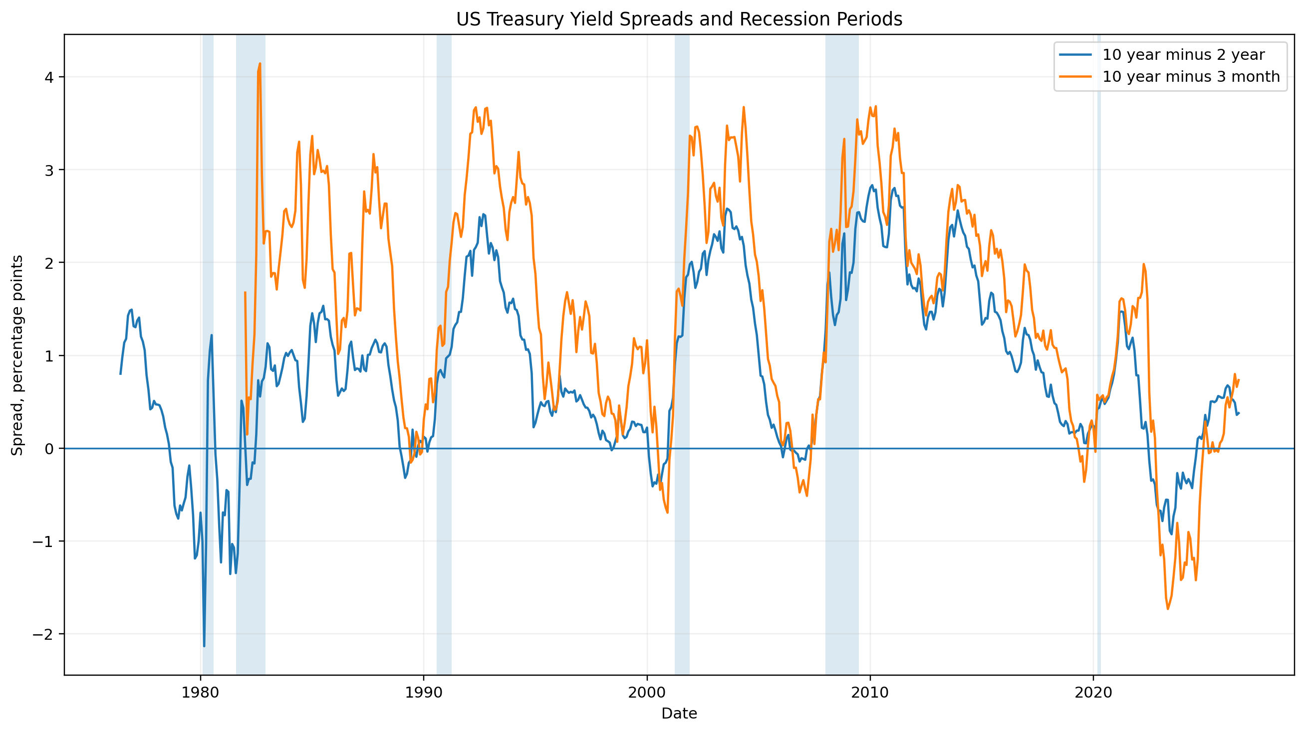
The main chart makes the basic pattern easy to see. Both spreads fall below zero before several recessions, but the timing and depth are different. The zero line is the key threshold. Recession shading is based on USREC.
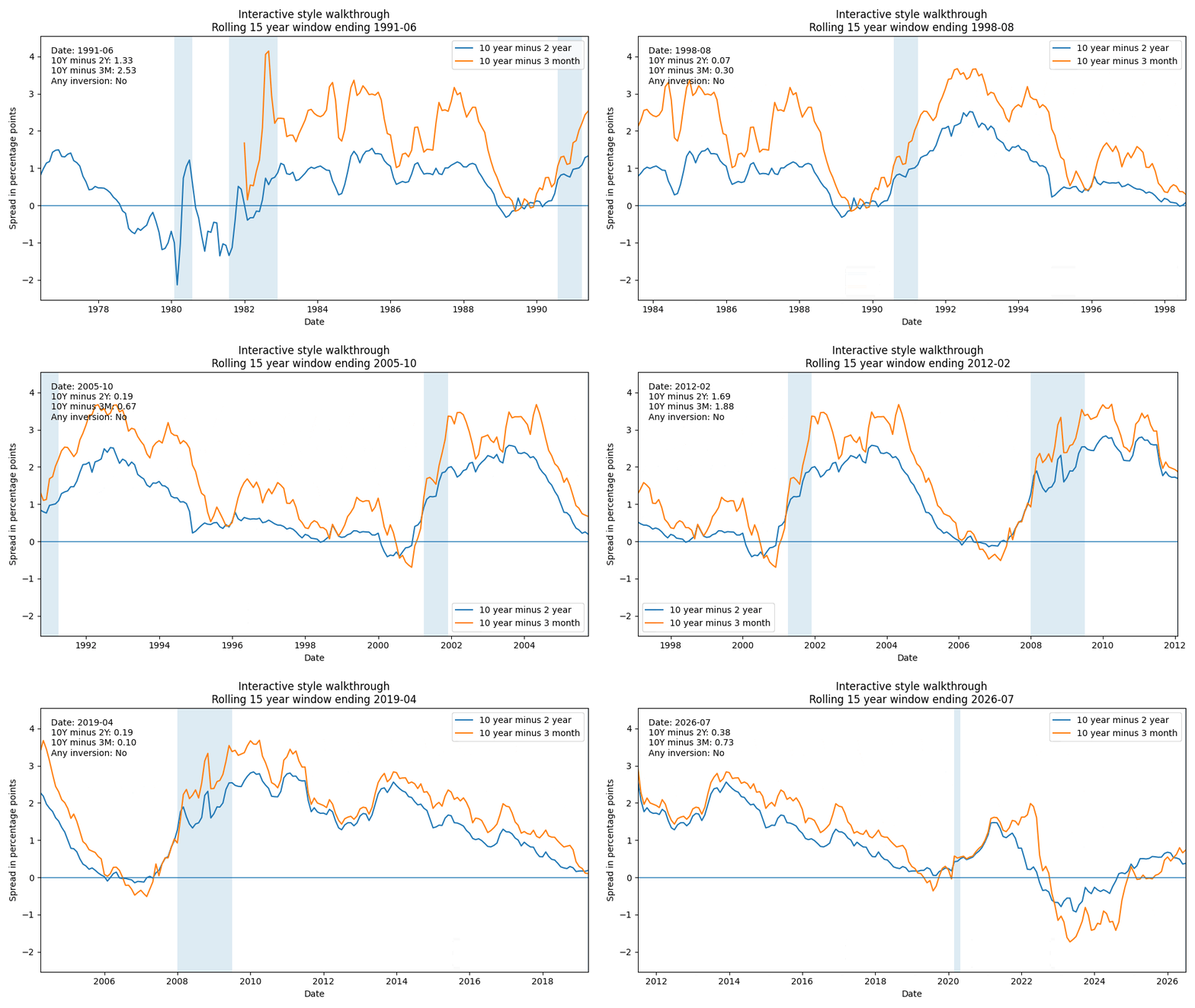
For a web article, the interactive Plotly version lets readers hover over each month and use a range slider. The HTML file that comes with this article also includes a true animation that reveals the history over time. The Word version uses the static chart because Word cannot play Plotly frames like a web browser.
Interactive chart
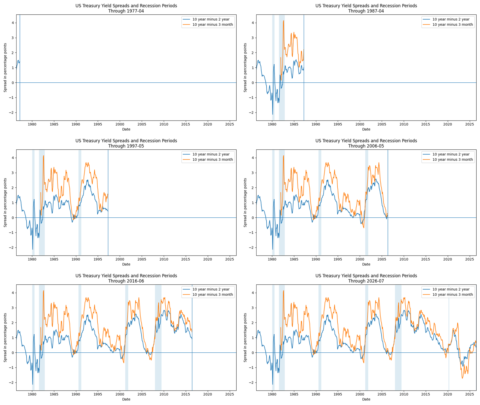
Animated history
Use Play to reveal the monthly spread history over time. This animation is designed to show how an inversion can form before a recession window rather than to decorate the page.
import matplotlib.pyplot as plt

plot_data = spreads[["T10Y2Y", "T10Y3M"]].copy()

fig, ax = plt.subplots(figsize=(12, 6))
ax.plot(plot_data.index, plot_data["T10Y2Y"], label="10 year minus 2 year")
ax.plot(plot_data.index, plot_data["T10Y3M"], label="10 year minus 3 month")
ax.axhline(0, linewidth=1)

rec = recession.fillna(0).astype(int)
starts = rec.index[rec.eq(1) & rec.shift(1, fill_value=0).eq(0)]
ends = rec.index[rec.eq(0) & rec.shift(1, fill_value=0).eq(1)]

for start, end in zip(starts, ends):
    ax.axvspan(start, end, alpha=0.15)

ax.set_title("US Treasury Yield Spreads and Recession Periods")
ax.set_ylabel("Spread, percentage points")
ax.legend()
plt.tight_layout()
plt.show()
Interactive Plotly version for the web
For production, add recession rectangles to the Plotly chart using the same start and end dates used for the Matplotlib shading. The supplied HTML version already does this and includes a play button animation.
import plotly.graph_objects as go

fig = go.Figure()
for series_id, label in [
    ("T10Y2Y", "10 year minus 2 year"),
    ("T10Y3M", "10 year minus 3 month"),
]:
    fig.add_trace(go.Scatter(
        x=spreads.index,
        y=spreads[series_id],
        mode="lines",
        name=label,
    ))

fig.add_hline(y=0, line_width=1)
fig.update_xaxes(rangeslider_visible=True)
fig.update_layout(
    title="Interactive US Yield Curve Recession Indicator",
    yaxis_title="Spread, percentage points",
    hovermode="x unified",
)
fig.show()
Compare the 10 year 2 year and 10 year 3 month spreads
The two spreads tell a similar story, but they are not interchangeable. T10Y2Y has a longer sample, starting in 1976. That gives it more recession events to test. Its baseline recall is 83.3 percent because the monthly average did not turn negative in the 6 to 24 month window before the 2020 recession.
T10Y3M starts in 1982, so it has fewer eligible recession starts. Within that shorter sample, it covered all four. This lines up with the research tradition that gives the 10 year minus 3 month spread special attention for recession forecasting.
Precision is not dramatically different under the one month baseline once recent open signals are handled correctly. T10Y2Y is 72.7 percent and T10Y3M is 71.4 percent. When we require two consecutive inverted months, both improve, and T10Y2Y reaches 87.5 percent while T10Y3M reaches 83.3 percent.
So which one is better? In this test, T10Y3M has stronger recession coverage, while T10Y2Y has more history and slightly higher precision under the two month persistence rule. That is a more useful conclusion than declaring one spread universally superior.
What an inverted yield curve can affect in the economy
An inverted curve is first a market signal. It often appears when short rates are high relative to longer rates and investors expect weaker growth or lower policy rates later. Those expectations can change business and household behavior before official recession data arrive.
Monetary conditions can feel tighter. High short rates raise financing costs for many borrowers. If companies face expensive working capital or refinancing, some may delay hiring, equipment purchases, or expansion plans.
Bank lending can also come under pressure. Banks do not simply borrow at one short rate and lend at one long rate, so the real balance sheet is more complex. Still, Federal Reserve research has discussed how a flatter or inverted curve can squeeze some lending margins and can be linked with tighter loan standards. Less credit creation can slow spending and investment.
Businesses may become more cautious. A curve inversion often arrives with concern about future demand. Firms can respond by protecting cash, slowing inventory growth, or delaying large projects. Consumers can also become more cautious when borrowing costs are high and job growth looks less certain.
None of this means the inversion itself mechanically causes every recession. The curve can reflect policy, inflation, growth expectations, term premiums, and demand for safe assets. In some periods, those forces may matter more than in others.
Limits, false signals, and timing risk
The biggest limit is timing. A useful signal can arrive far too early for exact forecasting. In the baseline true positive episodes, median lead time was 15.5 months for T10Y2Y and 10 months for T10Y3M. That is helpful for risk awareness, but not for choosing a precise month to expect a downturn.
False positives are real. The 1998 T10Y2Y monthly inversion did not lead to a recession inside the 6 to 24 month window. The major 2022 inversion also did not lead to an NBER recession start inside that completed window. For T10Y3M, the February 2020 one month inversion was too close to the recession start to pass the rule, while the November 2022 episode did not produce a recession start inside 24 months.
Recent signals can be unresolved. The 2025 T10Y3M inversions are still open in this backtest because July 2026 does not give them a full 24 month outcome window. Calling them false positives now would use an unfair amount of future information.
The economic meaning can also change across eras. Inflation regimes, Federal Reserve policy, quantitative easing, investor demand for safe assets, and shifts in the term premium can change the shape of the curve. Federal Reserve research has found that the plain term spread still contains useful information, but also shows why the signal should be read with other financial and economic data.
The 2020 recession is another warning about simple stories. The yield curve did invert in 2019, but the recession was tied to the sudden pandemic shock. A historical match does not prove that the curve predicted the exact cause of the downturn.
What the test tells us
This yield curve recession indicator Python test supports a careful conclusion. Yield curve inversion has been a useful US recession warning signal, especially when the 10-year 3-month spread is used and when very short inversion episodes are filtered out.
But the signal is not a timer. It can arrive many months early. It can produce false positives. It can also remain unresolved for a long period. The best use is as one part of a broader recession dashboard that also tracks employment, credit conditions, inflation, real activity, and financial stress.
Frequently asked questions
Which yield spread is most useful for recession forecasting?
The 10-year minus 3-month spread has a strong research record and covered all four eligible recession starts in this article's post-1982 sample. The 10-year minus 2-year spread has a longer FRED history and remains useful as a market signal.
How long after a yield curve inversion can a recession begin?
There is no fixed delay. This tutorial uses 6 to 24 months as the baseline window. In the scored true positive episodes, the median lead was 15.5 months for T10Y2Y and 10 months for T10Y3M.
Does every inverted yield curve cause a recession?
No. An inversion is an indicator, not a guaranteed cause. The backtest contains false-positive episodes, and economic shocks can arrive for reasons that are not contained in the yield curve.
Why use USREC instead of making my own recession dates?
USREC is a monthly FRED series based on NBER business cycle dating. It gives a reproducible recession label and makes it easier to align the yield spread with monthly recession periods.
Can I build a recession probability model in Python instead of a zero threshold rule?
Yes. A common next step is a probit or logistic model that maps the spread to a recession probability. Start with the simple zero threshold first, because it is easy to audit and avoids hiding the main result inside a fitted model.
Methodology note
Series IDs: T10Y2Y, T10Y3M, and USREC. Data source: Federal Reserve Economic Data. Spread frequency: daily, converted to monthly mean. Recession frequency: monthly. Inversion threshold: spread below zero. Baseline persistence: one monthly observation. Robustness rules: two and three consecutive inverted months, with the signal confirmed in the final required month. Baseline forecast window: recession start 6 to 24 months after the signal. Sensitivity window: 6 to 18 months. Recent signals are left open until the full maximum lead window is observed. Signals that begin during an existing recession are not scored as new forecasts.
Sources
- Federal Reserve Bank of St. Louis, FRED T10Y2Y: https://fred.stlouisfed.org/series/T10Y2Y
- Federal Reserve Bank of St. Louis, FRED T10Y3M: https://fred.stlouisfed.org/series/T10Y3M
- Federal Reserve Bank of St. Louis, FRED USREC: https://fred.stlouisfed.org/series/USREC
- National Bureau of Economic Research, Business Cycle Dating: https://www.nber.org/research/business-cycle-dating
- Federal Reserve Board, Predicting Recession Probabilities Using the Slope of the Yield Curve: https://www.federalreserve.gov/econres/notes/feds-notes/predicting-recession-probabilities-using-the-slope-of-the-yield-curve-20180301.html
- Federal Reserve Bank of San Francisco, Information in the Yield Curve about Future Recessions: https://www.frbsf.org/research-and-insights/publications/economic-letter/2018/08/information-in-yield-curve-about-future-recessions/
- Federal Reserve Bank of New York, The Yield Curve as a Predictor of U.S. Recessions: https://www.newyorkfed.org/research/current_issues/ci2-7.html
- Federal Reserve Bank of St. Louis, Can an Inverted Yield Curve Cause a Recession?: https://www.stlouisfed.org/on-the-economy/2018/december/inverted-yield-curve-cause-recession
Suggested internal links
- forecast U.S. GDP in Python
- Regional Price Parities by State: 2024 Cost Comparison
- U.S. Treasury Fiscal Data API: Debt Analysis in Python
- Analyze the U.S. unemployment rate in Python
- Real Wage Growth Calculator: Python Tutorial
Disclaimer
This tutorial is for education only and is not investment advice.
Editor checklist
- SEO: exact H1 appears once, primary keyword is used naturally, meta title and description are ready.
- Factual accuracy: FRED series IDs, sample dates, and recession dating method are stated.
- Code execution: run the notebook once with a live internet connection and confirm the printed latest dates.
- Chart export: save a high-resolution PNG for non-web use and keep the interactive Plotly chart in the HTML article.
- Mobile tables: use horizontal scrolling for the episode tables on small screens.
- Links: verify FRED, NBER, Federal Reserve Board, New York Fed, and San Francisco Fed links before publishing.
Downloads
Files attached to this article for your reference.