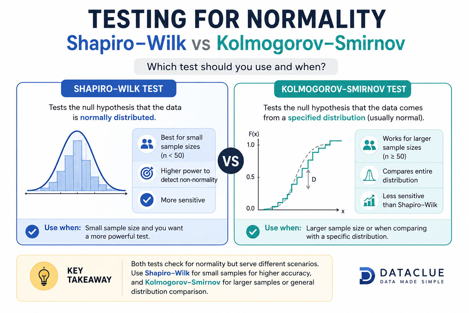
In this guide

• How to choose between Shapiro-Wilk, Kolmogorov-Smirnov, Lilliefors, and Anderson-Darling
• What normality tests actually assess and how to interpret p-values
• Why Q-Q plots should accompany formal tests
• How to run the tests in Python, R, and SPSS
• Common mistakes, reporting templates, and practical alternatives when data are non-normal

1. Shapiro-Wilk vs Kolmogorov-Smirnov: the main decision

When the objective is specifically to test whether a sample is consistent with a normal distribution, the Shapiro-Wilk test is usually the better first choice. It was designed for normality testing and generally has stronger power to detect departures from normality than the ordinary Kolmogorov-Smirnov test.

The Kolmogorov-Smirnov test, commonly called the KS test, has a broader purpose. It compares an empirical cumulative distribution with a fully specified theoretical distribution, or compares the distributions of two independent samples.

Critical limitation Standard one-sample KS p-values are not valid when the mean, standard deviation, or other distribution parameters have been estimated from the same data. Use Shapiro-Wilk, a Lilliefors correction, or a calibrated simulation or bootstrap procedure.

Research objective	Recommended approach
Test whether a sample is normally distributed	Shapiro-Wilk plus a Q-Q plot
Test residual normality in regression or ANOVA	Q-Q plot of residuals, supported by Shapiro-Wilk
Compare a sample with a fully specified continuous distribution	One-sample Kolmogorov-Smirnov
Compare two independent continuous distributions	Two-sample Kolmogorov-Smirnov
Test normality after estimating mean and standard deviation	Shapiro-Wilk or Lilliefors, not an unadjusted KS test
Detect departures mainly in the tails	Consider Anderson-Darling
Assess normality in a very large dataset	Emphasize plots, model diagnostics, and practical impact

Do not select a test using the simplistic rule “Shapiro-Wilk below 50 observations and KS above 50.” The research question and the parameter-estimation process matter more than that threshold.

2. What does testing for normality mean?

A normality test evaluates whether a sample is reasonably consistent with a normal distribution. The normal distribution is continuous, symmetric, and bell-shaped, with the mean, median, and mode located at the center.

Normality assumptions arise in procedures such as:

• t-tests
• analysis of variance (ANOVA)
• linear regression
• certain confidence intervals
• some forms of Pearson correlation inference
• classical process-control and measurement methods

Test the correct quantity In regression and ANOVA, the relevant assumption usually concerns model errors, which are evaluated through residuals. It normally does not require every predictor or every raw variable to be normally distributed.

Normality is only one part of model validity. Independence, appropriate specification, constant variance, measurement quality, and influential observations may be equally or more important.

3. Why normality testing matters

Normality can affect the accuracy of standard errors, confidence intervals, and p-values in some classical procedures. Serious skewness, heavy tails, outliers, or mixtures of populations may make conventional results unreliable, especially in small samples.

A significant normality test does not automatically invalidate a parametric analysis. Many methods remain reasonably robust under moderate non-normality, depending on sample size, group balance, the form and severity of the departure, influential observations, variance equality, and the objective of the analysis.

The practical question Do not ask only whether the distribution is perfectly normal. Ask whether the departure is serious enough to affect the planned analysis and its conclusions.

4. The Shapiro-Wilk test

The Shapiro-Wilk test is a formal test developed specifically to assess normality.

Hypotheses

• H₀: The sample comes from a normally distributed population.
• H₁: The sample does not come from a normally distributed population.

W = [Σ aᵢx₍ᵢ₎]² / Σ(xᵢ − x̄)²

The test compares ordered sample values with the pattern expected from normal order statistics. A W value closer to 1 usually indicates closer agreement with normality, but there is no universal cutoff. Interpret the p-value together with graphical diagnostics.

How to interpret the p-value

Result	Statistical decision	Correct interpretation
p < 0.05	Reject H₀	The sample provides evidence against normality.
p ≥ 0.05	Fail to reject H₀	The test did not find sufficient evidence against normality.

Interpretation warning A p-value above 0.05 does not prove that a population is normal. A p-value below 0.05 does not measure the size or practical importance of the departure.

Example report: “The Shapiro-Wilk test did not provide evidence of a departure from normality, W = 0.976, p = 0.312. The Q-Q plot was also approximately linear, supporting the normality assumption.”

5. The Kolmogorov-Smirnov test

The Kolmogorov-Smirnov test is a general goodness-of-fit test based on cumulative distribution functions. For a one-sample test, the statistic is the largest absolute difference between the empirical cumulative distribution function Fₙ(x) and the reference cumulative distribution function F₀(x).

D = maxₓ |Fₙ(x) − F₀(x)|

A larger D indicates a greater discrepancy between the observed and reference distributions.

One-sample KS test

Use the one-sample KS test when the continuous reference distribution and all its parameters are specified independently of the sample being tested. Examples include a normal distribution with a prespecified mean and standard deviation, an exponential distribution with a known rate, or a uniform distribution with known limits.

Two-sample KS test

Use the two-sample KS test to evaluate whether two independent samples appear to come from the same continuous distribution. Unlike a t-test, it is not restricted to differences in means and may detect differences in location, spread, or shape.

The parameter-estimation problem

1. Calculate the sample mean.
2. Calculate the sample standard deviation.
3. Use those values to define the reference normal distribution.
4. Apply the ordinary one-sample KS p-value.

Why this workflow is invalid Estimating parameters from the same sample changes the null distribution of the KS statistic. Standard KS critical values and p-values are therefore no longer valid.

Lilliefors correction

The Lilliefors test modifies the KS procedure for cases in which parameters such as the population mean and variance are unknown and estimated from the sample. It retains the maximum-distance idea but uses corrected critical values or p-value calculations.

Practical recommendation Lilliefors is useful when a KS-style normality test is required, but it should not automatically replace Shapiro-Wilk. For routine normality assessment, Shapiro-Wilk is generally more sensitive.

6. Comparison of the tests

Feature	Shapiro-Wilk	Kolmogorov-Smirnov
Main purpose	Test normality	Test goodness of fit or compare two distributions
Normality-specific	Yes	No
Relative power for normality	Generally higher	Generally lower than Shapiro-Wilk
Reference parameters	Handled within the procedure	Must be fully specified for an ordinary one-sample test
Estimated parameters	Built into normality-testing framework	Requires Lilliefors, bootstrap, or another adjustment
Tail sensitivity	Detects several forms of non-normality	Ordinary KS is less sensitive in the tails
Two-sample comparison	No	Yes
Best use	Routine normality assessment	Fully specified goodness-of-fit tests and two-sample comparisons

7. Sample size: what changes and what does not

There is no universal sample-size rule that requires Shapiro-Wilk below 50 observations and KS above 50. Software limits and p-value approximations should not be confused with statistical principles.

Small samples

Formal tests may have limited power in small samples. A non-significant result can occur even when the underlying population is noticeably non-normal. Combine the test with:

• a Q-Q plot
• a histogram where informative
• knowledge of the measurement process
• checks for extreme or influential observations

Large samples

With a large sample, formal tests may detect minor imperfections that are statistically significant but practically unimportant. Focus on:

• Q-Q plots and residual diagnostics
• skewness and tail behavior
• influential observations
• sensitivity analyses
• robust standard errors or robust models
• whether conclusions change under reasonable alternatives

Do not switch automatically A large sample is not, by itself, a reason to replace Shapiro-Wilk with the ordinary KS test.

8. Why a Q-Q plot should accompany a normality test

A normal Q-Q plot compares observed sample quantiles with the quantiles expected under a normal distribution. When the points follow an approximately straight line, the distribution is reasonably consistent with normality.

Pattern	Possible interpretation
S-shaped curvature	Possible skewness
Departures at both ends	Heavy or light tails
One isolated point	Possible outlier
Separate clusters or abrupt bends	Possible mixtures or subgroups
Systematic curvature	Broader distributional misspecification

A Q-Q plot shows the nature of a departure, whereas a single p-value only signals whether the evidence is statistically unusual under the null hypothesis.

9. Recommended workflow

1. Identify the actual assumption: raw values, group values, paired differences, model errors, or residuals.
2. Check data quality: impossible values, missing patterns, duplicates, limits, rounding, and influential observations.
3. Inspect graphical diagnostics: Q-Q plot, histogram, boxplot, and model-specific residual plots.
4. Apply the appropriate test: Shapiro-Wilk, Lilliefors, one-sample KS, two-sample KS, or Anderson-Darling.
5. Interpret the result correctly: use “reject” or “fail to reject,” not “prove” or “accept” normality.
6. Assess practical consequences and select a response that matches the research question.

Outlier rule Do not delete an observation solely to obtain a non-significant p-value. Any exclusion should have a defensible scientific, procedural, or data-quality justification.

10. Software implementation

Python

Shapiro-Wilk test

import numpy as np from scipy import stats data = np.array([12.1, 11.7, 12.8, 13.0, 12.4, 11.9, 12.6, 12.3, 12.7, 12.0]) result = stats.shapiro(data) print(f"W = {result.statistic:.4f}") print(f"p-value = {result.pvalue:.4f}")

Normal Q-Q plot

import matplotlib.pyplot as plt from scipy import stats stats.probplot(data, dist="norm", plot=plt) plt.title("Normal Q-Q Plot") plt.show()

Lilliefors test

from statsmodels.stats.diagnostic import lilliefors statistic, p_value = lilliefors(data, dist="norm") print(f"Lilliefors statistic = {statistic:.4f}") print(f"p-value = {p_value:.4f}")

One-sample KS test with prespecified parameters

from scipy import stats # Specify these independently of the tested sample. mu_0 = 12.5 sigma_0 = 0.6 result = stats.kstest(data, "norm", args=(mu_0, sigma_0)) print(f"D = {result.statistic:.4f}") print(f"p-value = {result.pvalue:.4f}")

Python warning Do not replace mu_0 and sigma_0 with data.mean() and data.std() and then interpret the ordinary KS p-value as valid. Use Lilliefors or another calibrated procedure.

R

x <- c(12.1, 11.7, 12.8, 13.0, 12.4, 11.9, 12.6, 12.3, 12.7, 12.0) shapiro.test(x) qqnorm(x) qqline(x, col = "red") library(nortest) lillie.test(x) mu_0 <- 12.5 sigma_0 <- 0.6 ks.test(x, "pnorm", mean = mu_0, sd = sigma_0)

SPSS

1. Select Analyze.
2. Choose Descriptive Statistics.
3. Select Explore.
4. Move the relevant outcome or residual variable into the Dependent List.
5. Select Plots and choose Normality plots with tests.
6. Select a histogram if required, then click Continue and OK.

The output includes a normal Q-Q plot, a detrended Q-Q plot, the Shapiro-Wilk test, and a Kolmogorov-Smirnov statistic with the Lilliefors significance correction.

SPSS interpretation The tests may produce different p-values because they use different statistics and sensitivities. For routine normality assessment, give greater weight to Shapiro-Wilk and the Q-Q plot rather than selecting whichever result supports a preferred conclusion.

11. Common mistakes

1. Testing every raw variable

Regression does not require all predictors to be normally distributed. Examine the relevant residuals and model assumptions.

2. Using KS with sample-estimated parameters

This produces an invalid ordinary KS p-value unless a suitable correction or resampling procedure is used.

3. Treating p ≥ 0.05 as proof of normality

A non-significant result is a failure to reject normality, not confirmation of exact normality.

4. Treating p < 0.05 as automatic failure

A significant result should lead to investigation, not an automatic switch to a nonparametric method.

5. Choosing a test only from sample size

The purpose of the test and the parameter-estimation process matter more than the outdated 50-observation rule.

6. Ignoring graphical diagnostics

A p-value cannot show whether the issue is skewness, heavy tails, an outlier, or a mixture.

7. Removing outliers to obtain normality

Exclusions must be based on data quality, predefined criteria, or scientific justification.

8. Testing residuals from a misspecified model

Non-normal residuals may reflect missing nonlinear terms, omitted groups, unequal variance, dependence, or an unsuitable outcome distribution.

9. Applying ordinary KS to discrete or heavily rounded data

Standard KS theory assumes continuity, and ties can materially affect p-values.

12. When to consider Anderson-Darling

The Anderson-Darling test is another goodness-of-fit procedure. It gives greater weight to discrepancies in the tails than the ordinary KS test and may be useful in:

• financial return analysis
• reliability and failure-time analysis
• environmental extremes
• quality-control measurements
• risk modeling

13. What to do when data are not normal

A significant normality test should not trigger an automatic response. First determine why the data depart from normality and whether that departure affects the intended analysis.

Continue with the parametric method

Reasonable when the deviation is mild, the method is robust in the relevant setting, group sizes are adequate and balanced, there are no highly influential observations, and sensitivity analyses support the same conclusion.

Transform the outcome

Logarithmic, square-root, or Box-Cox transformations may be appropriate when they reflect the measurement scale or data-generating process. Do not transform merely to force p > 0.05.

Use a model suited to the outcome

Examples include logistic models for binary outcomes, Poisson or negative-binomial models for counts, gamma models for positive skewed values, survival models for time-to-event data, and mixed-effects models for clustered observations.

Use robust or resampling methods

Depending on the objective, consider robust standard errors, bootstrap confidence intervals, permutation tests, robust regression, trimmed-mean procedures, or rank-based methods.

14. How to report a normality assessment

When normality appears reasonable The normality of the model residuals was assessed using a Q-Q plot and the Shapiro-Wilk test. The Q-Q plot showed no substantial systematic departure from linearity, and the Shapiro-Wilk test was not significant, W = 0.982, p = 0.214. The normality assumption was therefore considered reasonable for the planned analysis.

When normality is rejected but the analysis is retained The Shapiro-Wilk test indicated a departure from normality, W = 0.961, p = 0.018. Inspection of the Q-Q plot showed a mild departure in the upper tail without influential outliers. Because group sizes were balanced and the primary conclusions were unchanged in a robust sensitivity analysis, the planned parametric analysis was retained.

When a robust alternative is used The residual distribution showed substantial right skew and several influential observations. The Shapiro-Wilk test rejected normality, W = 0.842, p < 0.001. A robust analysis was therefore used, and its assumptions and estimates were examined separately.

Replace the example statistics with the actual results from the study. Report the tested quantity, test statistic, p-value, visual evidence, and resulting analytical decision.

15. Frequently asked questions

Is Shapiro-Wilk better than Kolmogorov-Smirnov?

For normality testing, Shapiro-Wilk is generally the better first choice because it is designed for normality and usually has greater power. KS remains useful for fully specified distributions and two-sample distribution comparisons.

Which normality test should I use for a sample larger than 50?

Do not choose solely from the number 50. For large datasets, combine a Q-Q plot, residual diagnostics, and practical assessment rather than relying only on a formal p-value.

What does p < 0.05 mean in a Shapiro-Wilk test?

The sample provides evidence against the null hypothesis of normality at the chosen significance level. It does not identify the form or practical importance of the departure.

What does p > 0.05 mean?

The test did not find sufficient evidence to reject normality. It does not prove that the population is exactly normal.

Should normality be tested on raw data or residuals?

It depends on the model. For regression and ANOVA, the relevant normality assumption generally concerns errors, evaluated through model residuals.

Can I use KS after calculating the sample mean and standard deviation?

Not with the ordinary KS p-value. Use Shapiro-Wilk, Lilliefors, or a properly calibrated simulation or bootstrap approach.

Why do SPSS Shapiro-Wilk and KS results differ?

The tests use different statistics and sensitivities. SPSS also applies a Lilliefors significance correction to its KS normality test. Interpret both alongside Q-Q plots.

Is a histogram enough?

A histogram is useful but depends on bin width and may be difficult to interpret in small samples. A normal Q-Q plot is usually more informative.

Is normality required for every statistical test?

No. Assumptions vary by method, and robust, generalized, nonparametric, and resampling procedures are available when classical assumptions are inappropriate.

Final recommendation

1. Identify the observations or residuals for which normality is relevant.
2. Check data quality and influential observations.
3. Inspect a normal Q-Q plot.
4. Use Shapiro-Wilk as the main formal normality test.
5. Interpret the p-value as evidence, not proof.
6. Evaluate whether any departure is practically important.
7. Use a robust or alternative model only when it better answers the research question.

Bottom line Use the Kolmogorov-Smirnov test when comparing a sample with a fully specified continuous distribution or comparing two independent continuous samples. When parameters are estimated from the sample, do not use an ordinary one-sample KS p-value. The best assessment combines graphical evidence, a suitable test, sample size, research design, and the consequences for the intended analysis.

References and authoritative documentation

1. SciPy: scipy.stats.shapiro documentation

2. SciPy: scipy.stats.kstest documentation

3. NIST/SEMATECH: Kolmogorov-Smirnov Goodness-of-Fit Test

4. R Core Team: Shapiro-Wilk Normality Test

5. R Core Team: Kolmogorov-Smirnov Tests

6. Statsmodels: Lilliefors Test

7. NIST/SEMATECH: Normal Probability Plot

8. NIST/SEMATECH: Anderson-Darling Test