Time Series Models: Types, Uses and Model Selection

Time series models analyze observations recorded in chronological order to identify temporal patterns and forecast future values. They are appropriate when timing matters and today’s value may depend on earlier values, recurring calendar effects, external variables, or changing operating conditions.

The practical goal is not to find the most sophisticated algorithm. It is to build the simplest forecasting system that captures the useful structure, uses information genuinely available at prediction time, and performs reliably when tested on later periods.

What Are Time Series Models in Simple Terms?

A Simple Definition of a Time Series Model

A time series model is a statistical or computational method for data indexed by time. It can describe how a sequence behaves, estimate relationships among past and present observations, detect unusual changes, or produce forecasts for future periods.

Daily sales, hourly electricity demand, monthly revenue, minute-by-minute website traffic, and sensor readings are all time series. The target may be one variable, such as units sold, or several connected variables, such as sales, price, promotions, and local weather.

How Time Series Data Differs From Standard Tabular Data

The order of rows is meaningful. A sale recorded today may be related to yesterday, the same weekday last week, and the corresponding holiday period last year. Shuffling the rows can destroy that structure and can also allow future information to influence training.

This is why ordinary random cross-validation is usually inappropriate for forecasting. Time-aware splitting keeps training observations earlier than the validation observations, which better represents deployment. scikit-learn

Time Series Analysis vs Time Series Forecasting

Time series analysis studies historical structure, including trend, seasonality, autocorrelation, volatility, anomalies, and structural changes. Time series forecasting uses that structure, together with any relevant external information, to estimate unknown future values.

The distinction matters because not every time-dependent task is a forecast. A cybersecurity team may detect an abnormal traffic spike without predicting next month’s traffic, while an inventory team needs future demand estimates before it places an order.

A Simple Forecasting Example

Suppose a bakery needs tomorrow’s demand. A basic forecast may repeat today’s sales. A seasonal-naive forecast may use sales from the same weekday last week. A feature-rich model could also use recent demand, scheduled promotions, holidays, temperature forecasts, and local events.

The most suitable approach depends on the decision. Preparing bread for tomorrow requires a short horizon and fast updates; planning a new production line requires longer-term scenarios and wider uncertainty ranges.

Why Time Series Models Matter

Forecasting Demand, Sales, and Revenue

Forecasts support decisions that must be made before the outcome is known. Retailers order inventory, call centers schedule employees, utilities prepare generation capacity, and finance teams plan cash requirements before actual demand or revenue arrives.

Historical data is useful when the future retains some relationship with the past. Forecastability usually improves when recurring patterns are stable, relevant predictors are available, and the forecast horizon is not excessively long.

Detecting Patterns and Operational Anomalies

A model can reveal a gradual trend, a recurring weekly cycle, or an observation that falls outside the expected range. The unusual value may represent fraud, equipment failure, a successful promotion, a reporting error, or a genuine shift in behavior. The model flags the departure; domain knowledge determines what it means.

Supporting Inventory, Staffing, and Budget Decisions

Forecast error has a business cost. Underforecasting may cause stockouts, missed sales, or understaffing. Overforecasting may create waste, excess inventory, idle capacity, or unnecessary labor expense. The model should therefore be judged by the decision it supports, not only by an abstract accuracy score.

Communicating Forecast Uncertainty

A point forecast gives one value, while a prediction interval gives a plausible range. A forecast of 1,000 orders is far more actionable when the likely range is 960–1,040 than when it is 500–1,500. Forecasting guidance recommends intervals because they make uncertainty visible instead of hiding it behind one number. Forecasting: Principles and Practice

Core Components of Time Series Data

Trend, Seasonality, Cycles, and Residual Variation

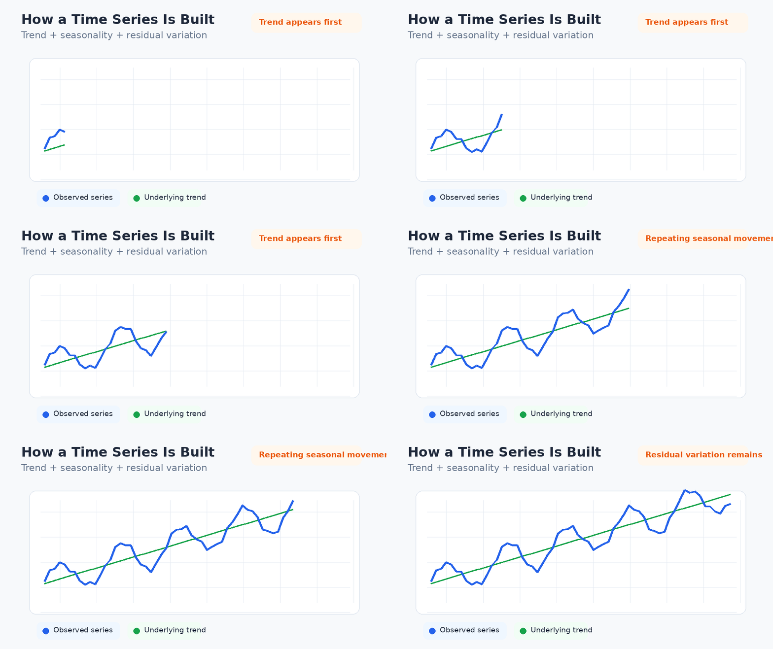
Trend is the long-term direction of the series. Seasonality is a recurring pattern tied to a known period, such as hour of day, day of week, or month of year. Cycles are broader rises and falls without a fixed calendar period. Residual variation is what remains after the explainable structure has been modeled.

The components are diagnostic ideas rather than mandatory ingredients of every algorithm. Decomposition helps readers and practitioners see what the data contains before deciding how it should be modeled. Forecasting: Principles and Practice

Additive vs Multiplicative Structure

In an additive series, seasonal changes remain similar in absolute size. Demand may rise by roughly 200 units every December. In a multiplicative series, the seasonal effect grows with the level, such as a holiday increase of about 30 percent as the business expands.

The distinction affects transformations and model design. Logarithms can make multiplicative variation easier to model, while methods such as exponential smoothing or Prophet can represent seasonal effects in different ways.

Essential Time Series Concepts Explained

Autocorrelation, Lags, and Partial Autocorrelation

Autocorrelation measures the relationship between a series and delayed versions of itself. In daily data, strong autocorrelation at lag seven may indicate that values resemble those from the same weekday one week earlier.

A lag feature is an earlier observation used as an input. Lag one is the previous period; lag seven is seven periods earlier. Partial autocorrelation estimates the direct relationship with a chosen lag after accounting for shorter lags. ACF and PACF plots can guide classical model specification, but they should not replace validation.

Stationarity

A stationary series has statistical properties that remain sufficiently stable over time. Its level, variation, and dependence structure do not systematically change with the observation date. Trend and seasonality commonly make an original series non-stationary.

Stationarity is especially important in ARIMA-style modeling, where differencing can remove changing levels or seasonal patterns. It is not a universal requirement for every forecasting algorithm; ETS, Prophet, tree-based methods, and neural networks represent temporal structure differently. Forecasting: Principles and Practice

Frequency, Granularity, and Forecast Horizon

Frequency describes how often observations are recorded. Granularity should match the decision: monthly data cannot reveal the hourly peaks needed for workforce scheduling, while second-by-second data may be unnecessarily noisy for an annual budget.

The forecast horizon is how far ahead the model predicts. Recent lags may be highly informative for tomorrow but much less useful for next year. Model performance should be evaluated at the same horizons used in the real workflow.

Univariate and Multivariate Time Series

A univariate series contains one modeled variable, such as daily revenue. A multivariate system tracks several evolving variables, such as sales, price, advertising, traffic, and weather. A model may also forecast one target with external regressors without jointly forecasting every input.

How to Test Whether a Time Series Is Stationary

Visual Diagnostics

A changing average level, widening variance, or evolving seasonal pattern may indicate non-stationarity. Line plots, rolling statistics, and decomposition views help reveal these changes, although the selected window and scale can affect what the chart appears to show.

The Augmented Dickey-Fuller Test

The Augmented Dickey-Fuller test evaluates a null hypothesis involving a unit root. Its p-value must be compared with a chosen significance level, such as 0.05. It is incorrect to claim that every p-value above zero proves non-stationarity or that the p-value must equal zero before the series can be treated as stationary. statsmodels

Rejecting the ADF null provides evidence against a unit root under the selected specification. It does not prove that every possible form of non-stationarity, seasonality, or structural change has disappeared.

The KPSS Test

The KPSS test starts from a different null hypothesis: level or trend stationarity, depending on the chosen specification. Using ADF and KPSS together can provide a more balanced diagnosis because agreement strengthens the conclusion and disagreement signals the need for closer inspection. statsmodels

How to Use the Results

Stationarity tests should inform model design rather than become a mechanical gate. A trend may be differenced, represented explicitly, or handled through a shorter training window. A structural break may require event variables or a new regime rather than repeated differencing.

How to Prepare Time Series Data for Modeling

Validate Timestamps and Data Frequency

Convert timestamps into one consistent format, sort them chronologically, identify duplicates, and confirm the time zone. Clarify whether each timestamp marks the start of a period, the end of a period, or an aggregate across the period.

Reindex the series to its expected frequency before creating lags. A missing row and a recorded zero are not equivalent: zero demand may represent no purchases, a stockout, or a closed store, while a missing value may represent a reporting failure.

Handle Missing Values and Outliers Carefully

Interpolation is reasonable only when the missing value can be inferred from nearby observations. An outlier should be investigated before removal. A data-entry error may need correction, but a promotion spike or system shutdown may be a real event that should remain visible or be modeled with an indicator.

Model or Transform Trend and Seasonality

ARIMA often uses differencing, ETS represents level, trend, and seasonality as evolving states, and Prophet uses an additive decomposition with configurable seasonal and holiday effects. Tree-based models usually receive lag, rolling, calendar, and event features instead.

Log or Box-Cox transformations can stabilize changing variance, but forecasts must be transformed back carefully. Scaling is often useful for neural networks and some linear models, while tree ensembles generally do not depend on feature scaling in the same way.

Prevent Data Leakage

Leakage occurs whenever model development uses information that would not have been available at the actual forecast date. Common sources include full-dataset scaling, centered moving averages, future-aware rolling statistics, revised historical records, and regressors observed only after the target period.

Preprocessing must be fitted inside each training window, not once on the full dataset. External variables must also be classified as known in advance, forecastable with uncertainty, or unavailable. A future promotion schedule can be used if it was genuinely fixed before the forecast; a realized competitor price recorded afterward cannot.

Main Types of Time Series Models

Baseline and Naive Forecasting Models

A naive forecast repeats the latest observation. A seasonal-naive forecast repeats the corresponding observation from the previous seasonal cycle. These models are not throwaway examples; they establish the minimum performance that added complexity must beat. Simple methods can be surprisingly effective. Forecasting: Principles and Practice

Classical Statistical Models

Classical methods include autoregression, ARIMA, exponential smoothing, state-space models, and vector autoregression. They are often strong choices for small or moderately sized datasets with structured patterns and a need for transparent assumptions.

Machine Learning Models

Machine learning usually reframes the sequence as supervised regression. Each row contains historical lags, rolling statistics, calendar variables, category attributes, and external predictors. Random Forest, XGBoost, and LightGBM can then model nonlinear interactions.

Deep Learning Models

Deep learning models learn sequence representations through recurrent units, convolutions, or attention. They become more attractive when the project contains many observations, many related series, complex covariates, or demanding multistep horizons.

Hybrid, Ensemble, Local, and Global Models

Hybrid systems combine different model families, while ensembles combine their forecasts. Local models are fitted separately to each series; global models learn across many related series. A global model may help low-volume products borrow information from categories, stores, or regions with similar behavior.

The M4 Competition evaluated 61 methods across 100,000 series and reinforced the value of empirical comparison rather than assuming that one family dominates. Forecast combinations also remain difficult to beat consistently. International Journal of Forecasting Forecasting: Principles and Practice

Classical Statistical Time Series Models

AR, MA, and ARMA

An autoregressive model predicts the current value from earlier values of the same series. An MA(q) model represents the current value through current and past error terms. ARMA combines both structures for a stationary series.

An MA(q) error model is not the same as moving-average smoothing. Smoothing averages nearby observations to expose a trend; an MA model describes dependence through residual shocks. Confusing the two leads to incorrect explanations and model choices.

ARIMA, SARIMA, and SARIMAX

ARIMA combines autoregression, differencing, and moving-average errors. Its notation is ARIMA (p, d, q), where p is the autoregressive order, d is the differencing order, and q is the moving-average order. Forecasting: Principles and Practice

SARIMA adds seasonal autoregressive, differencing, and moving-average terms, usually written as (p, d, q)(P, D, Q, s), where s is the seasonal period. SARIMAX adds external regressors such as price, holidays, promotions, or weather. Forecasting: Principles and Practice

The practical difficulty with external regressors is future availability. If the future predictor must itself be forecast, its uncertainty also affects the target forecast and may not be fully represented in a standard prediction interval.

Exponential Smoothing, Holt, and Holt-Winters

Simple exponential smoothing gives progressively less weight to older observations and is appropriate when there is no clear trend or seasonality. Holt’s method adds a trend component, while Holt-Winters adds seasonality. Damped trend variants reduce the chance of extending recent growth indefinitely.

Vector Autoregression

Vector autoregression models several related time series jointly so that lagged values of each variable may influence the others. The parameter count grows quickly as more variables and lags are added, making careful selection and sufficient data important.

Machine Learning Models for Time Series Forecasting

Turning a Sequence Into a Feature Table

A machine-learning forecasting dataset should represent what was known at each forecast origin. A row may include demand from one, seven, and 28 days earlier, recent rolling averages, weekday, month, scheduled promotions, and a weather forecast.

Lagged-feature examples in scikit-learn show both the supervised framing and the need for time-aware evaluation. The algorithm does not understand chronology automatically; the features and split strategy must preserve it. scikit-learn

Random Forest, XGBoost, and LightGBM

Random Forest can model nonlinear interactions and is relatively robust to noisy individual predictors. XGBoost and LightGBM often provide stronger feature-rich regression through sequential boosting and can be trained globally across many products, locations, or customers.

Their main limitations are feature-engineering effort, weak extrapolation beyond the training range, and the need for an explicit multistep strategy. A high-performing tree model can still fail if future lags are generated recursively without accounting for accumulating error.

Generalized Additive Models and Prophet

Generalized additive models use smooth functions to represent nonlinear trends and seasonal shapes while retaining more interpretability than many black-box methods.

Prophet is an additive forecasting procedure that models nonlinear trend, common seasonalities, and holiday effects. It is convenient for business calendars, but it is not automatically robust to every domain shift or irregular pattern. Its documentation recommends cross-validation and warns that aggregated weekly or monthly timestamps require careful holiday alignment. Prophet Prophet diagnostics Prophet non-daily data

When Machine Learning Is Worthwhile

Machine learning becomes more attractive when useful predictors interact nonlinearly, many related series can share one model, or calendar and category features carry substantial signal. A stable seasonal series may still be handled more efficiently by ETS or SARIMA, especially when interpretability and low maintenance matter.

Deep Learning Models for Time Series Data

RNN, LSTM, and GRU

Recurrent neural networks pass information from one time step to the next. LSTM networks add gates and an internal memory state to preserve or discard information over longer sequences. GRU networks use a simpler gated design with fewer components.

These architectures can capture nonlinear temporal relationships, but they normally need more data, tuning, and computing than classical methods. Neither LSTM nor GRU is universally superior; the relevant comparison is out-of-sample performance at the required horizons.

CNN and Temporal Convolutional Networks

One-dimensional convolutional networks detect local temporal shapes. Temporal convolutional networks use causal and often dilated convolutions so that a prediction depends only on present and past inputs while still covering a long history.

Transformers, TFT, and PatchTST

Transformers use attention to model relationships across positions in a sequence. They can process interactions in parallel, but standard attention can be expensive for long histories and does not guarantee better forecasts on small datasets.

The Temporal Fusion Transformer was designed for multihorizon problems containing static attributes, known future inputs, and variables observed only in the past. It combines recurrent processing, feature selection, gating, and attention. Temporal Fusion Transformer paper

PatchTST divides a series into patches and applies channel-independent transformer processing. The patching design reduces attention cost for a given lookback window and allows the model to attend to longer histories. PatchTST paper

When Deep Learning Justifies Its Complexity

Deep learning is most defensible when there are many related sequences, extensive historical data, complex covariates, or long multistep horizons. A single monthly series with a few years of observations rarely contains enough information to justify a transformer trained from scratch.

ARIMA vs Prophet vs XGBoost vs LSTM vs Transformers

Model family	Best suited to	Main advantage	Main limitation
ARIMA or SARIMA	Small, structured series with linear autocorrelation	Interpretable and statistically rigorous	Limited nonlinear and high-dimensional feature handling
Exponential smoothing	Stable level, trend, and seasonality	Fast, understandable, and effective	Limited support for complex external relationships
Prophet	Business data with calendar effects and trend changes	Convenient holiday and seasonality configuration	Can miss irregular interactions or changing regimes
XGBoost or LightGBM	Feature-rich or multi-series forecasting	Strong nonlinear interactions and global modeling	Requires deliberate feature engineering and leakage controls
LSTM or GRU	Large sequential datasets	Learns nonlinear temporal representations	Higher data, tuning, and maintenance needs
Transformers	Long, multivariate, or multihorizon sequences	Flexible attention and cross-series learning	Resource-intensive and not automatically superior

Which Model Is Most Interpretable?

Naive forecasts, ETS, structured regression, and modest ARIMA models are usually easiest to explain. Prophet also exposes recognizable trend, seasonal, and holiday components. Feature importance and attention scores can help with inspection, but they should not be treated as proof of causality.

Which Model Handles Seasonality Best?

Holt-Winters and SARIMA are strong starting points for stable fixed seasonal periods. Prophet is convenient for calendar seasonality and named events. Machine-learning and neural models may handle multiple interacting seasonalities when suitable features and sufficient data are available.

Which Model Works Best With External Variables?

SARIMAX and dynamic regression offer interpretable linear effects. Boosted trees are useful when predictors interact nonlinearly. TFT was designed for complex mixes of static attributes, known future inputs, and historically observed variables. In every case, the decisive question is whether those variables will exist at the forecast origin.

Which Models Need the Most Data?

Deep networks trained from scratch generally need the most data. Classical models can operate on shorter series, although very short histories still limit reliable parameter estimation and make honest validation difficult.

How to Choose the Right Time Series Model

Start With the Decision, Target, and Horizon

“Forecast sales” is not a complete objective. A usable objective might be: predict daily units for each product seven days ahead so replenishment orders can be placed. This statement defines the target, frequency, level of aggregation, horizon, and decision.

Assess Data Volume, Structure, and Predictor Availability

Count relevant seasonal cycles, not only rows. Two years of hourly data contains many observations but only two annual cycles. Check for trend, multiple seasonalities, intermittent demand, missing periods, and structural breaks.

Separate external variables into known future inputs, forecastable inputs, and unknown future inputs. Calendar dates and contracted promotions may be known. Weather can be forecast with error. Tomorrow’s realized competitor price may be unavailable.

Consider Interpretability, Cost, and Maintenance

The theoretically strongest model may be unrealistic if it cannot run within the decision window, requires unavailable infrastructure, or is too difficult for the team to maintain. A small reduction in average error may not justify higher latency, retraining cost, and operational risk.

Always Compare With a Baseline

A complex model must consistently outperform a relevant naive or seasonal-naive forecast on later periods. The conventional advice to “use deep learning for large data” is incomplete because data size alone does not show whether additional complexity creates operational value.

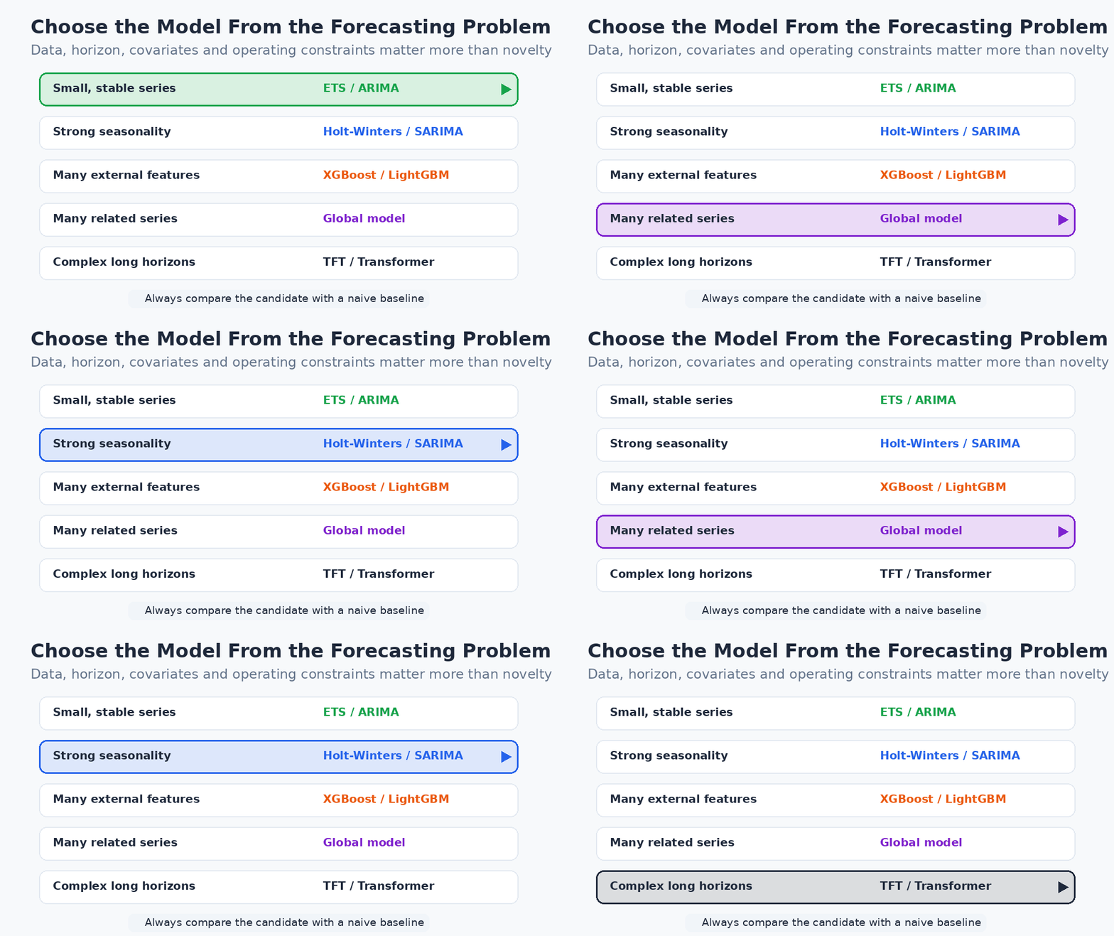
Forecasting situation	Recommended starting models
Small dataset with a stable pattern	Naive, seasonal naive, ETS, or ARIMA
Strong fixed seasonal cycles	Holt-Winters or SARIMA
Holidays and business events	Prophet or regression with event variables
Many useful external predictors	XGBoost, LightGBM, or SARIMAX
Many related products or locations	Global boosted-tree or global neural model
Complex multihorizon forecasting	TFT, TCN, or a transformer candidate
High interpretability requirement	ETS, ARIMA, or structured regression
Uncertain model choice	Several diverse candidates plus a simple ensemble

Step-by-Step Time Series Modeling Workflow

Define the Forecasting Contract

Specify the target, frequency, forecast horizon, update schedule, decision owner, acceptable latency, and cost of overforecasting versus underforecasting. This contract prevents the technical team from optimizing a metric that does not match the business decision.

Audit and Visualize the Data

Validate timestamps, units, definitions, missing intervals, outliers, and revisions. Plot both the full history and the recent operating period. Examine seasonal views, decomposition, autocorrelation, and meaningful subgroups.

Create Baselines and Candidate Models

Build naive and seasonal-naive forecasts first. Then select a small set of candidates whose assumptions match the data, such as ETS, SARIMA, Prophet, and a boosted-tree model. Testing every available algorithm adds cost without guaranteeing information gain.

Split Chronologically and Tune Safely

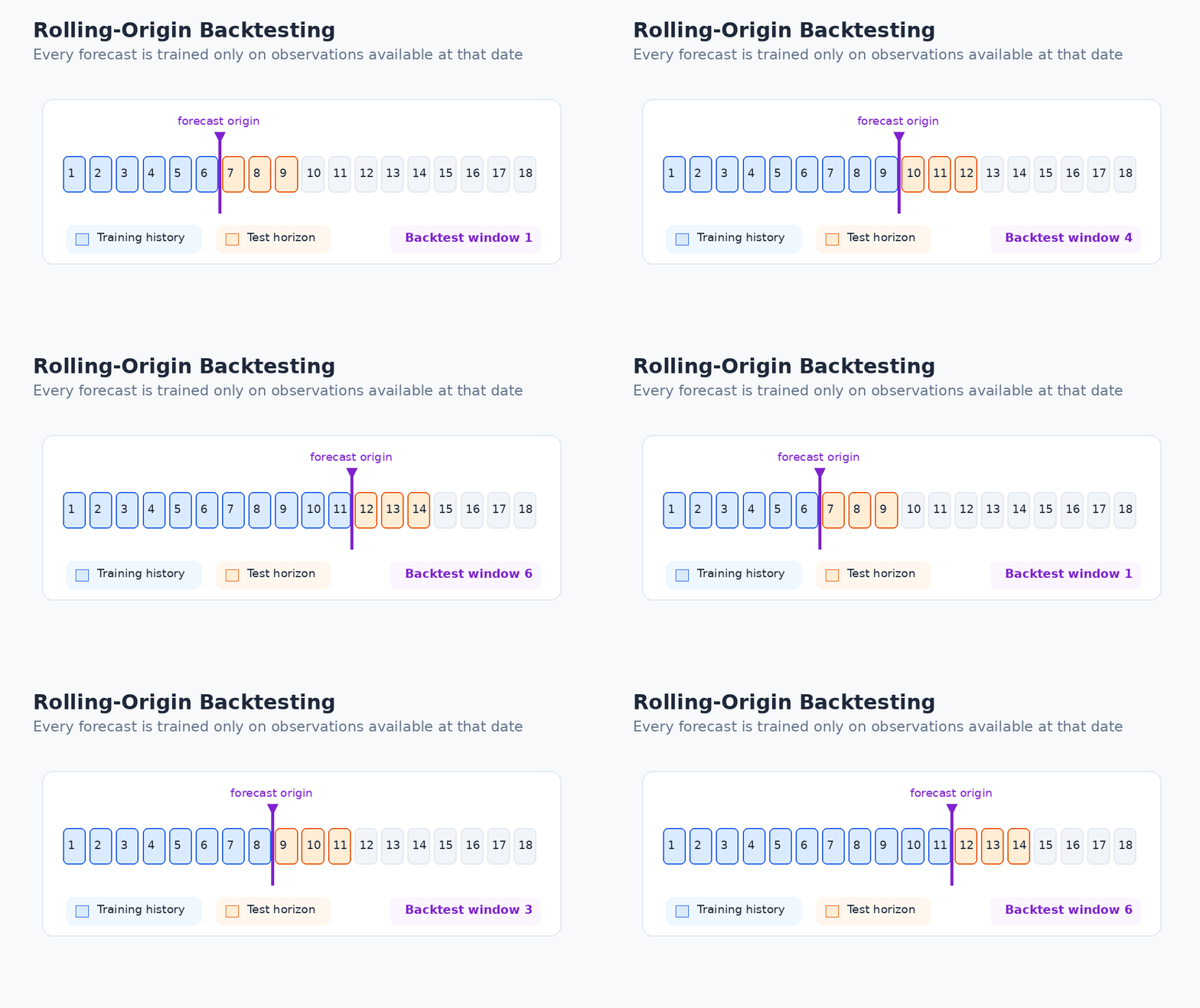
Reserve the latest period for final testing. Within the earlier history, tune models through rolling-origin validation. Fit scalers, imputers, transformations, feature selection, and model parameters separately inside each training window.

Compare Accuracy, Stability, and Uncertainty

Measure performance at each required horizon, not only as one average. Review bias, failure periods, prediction-interval coverage, training time, and sensitivity to structural change. A slightly better mean score may conceal severe misses during promotions or peak demand.

Deploy, Monitor, and Govern

Automate data checks, forecast generation, versioning, and metric reporting. Define alert thresholds, retraining rules, approval responsibilities, and rollback procedures. A forecasting pipeline is an operational system, not a model file.

How to Evaluate Time Series Models Correctly

Chronological Holdouts and Rolling-Origin Evaluation

A single chronological holdout trains on earlier observations and tests on a later block. It is simple, but the conclusion can depend heavily on the selected period. Rolling-origin evaluation repeats the exercise across several historical forecast dates and averages the errors. Forecasting: Principles and Practice

An expanding window retains all earlier observations as the origin advances. A sliding window keeps only the most recent fixed history, which may be more realistic when older regimes are no longer relevant.

MAE, RMSE, MAPE, and MASE

Mean absolute error measures average error in the target’s original units. Root mean squared error gives greater weight to large misses. MAPE expresses errors as percentages but becomes undefined at zero and unstable near zero.

Mean absolute scaled error compares the model with a naive benchmark and can be compared across series with different scales. The metric should reflect the business loss rather than convenience alone. Forecasting: Principles and Practice

Forecast Bias and Horizon-Specific Performance

A model can have acceptable average error while consistently forecasting too high or too low. Track bias and examine each lead time because a model may be strong at one day and poor at 28 days.

Prediction Intervals and Probabilistic Evaluation

A useful interval should be calibrated and reasonably narrow. If a nominal 90 percent interval contains only 60 percent of outcomes, it understates uncertainty. An extremely wide interval may achieve coverage while offering little operational guidance.

Match Evaluation to Business Cost

When underforecasting is more costly than overforecasting, symmetric metrics may select the wrong model. Quantile loss or a custom asymmetric cost can align the forecast with service levels, safety stock, staffing risk, or financial exposure.

What Time Series Models Can and Cannot Do

What They Can Predict Reliably

Forecasting works best when the process has recurring, measurable structure and the future resembles conditions represented in training. Stable seasonal demand, energy load, routine traffic, and repeated operational cycles are often more forecastable than one-off strategic events.

Why Uncertainty Grows Over Longer Horizons

As the horizon increases, recent lags lose direct relevance, recursive errors can accumulate, and more external conditions remain unknown. Prediction intervals should generally widen rather than imply equal confidence at every future step.

Unexpected Events and Structural Breaks

A model cannot reliably predict an event with no historical analogue or early explanatory signal. It may adapt after the event begins, but adaptation is not the same as advance prediction. New regulations, supply shocks, platform changes, and sudden consumer behavior can invalidate older relationships.

Prediction Is Not Causation

A variable can improve forecasts without causing the outcome. Website traffic and sales may move together because both respond to a campaign. Changing a correlated feature does not necessarily change the target.

The Limits of Stock-Price Forecasting

Historical-price forecasting is useful for teaching mechanics, but low test error does not establish a profitable trading strategy. Financial evaluation must account for transaction costs, execution delays, changing regimes, risk, and whether the information was available before the trade.

Common Time Series Modeling Mistakes

Training With Future Information

Leakage can enter through features, sequence construction, full-dataset normalization, revised records, or target-aware outlier treatment. Build a feature-availability record showing exactly when each input becomes known.

Ignoring Missing Periods and Calendar Details

Missing timestamps distort lags and seasonal periods. Time zones, daylight-saving changes, regional holidays, school calendars, trading days, and market-specific promotions can alter patterns. These are legitimate contextual signals, not random location keywords.

Using Random Cross-Validation

Random folds answer a different question from forecasting. They can train on later regimes and evaluate on earlier observations. Preserve temporal order unless the task has a carefully justified alternative design.

Failing to Beat a Naive Model

A sophisticated architecture that does not consistently beat a relevant baseline has not justified its cost. Accuracy should be measured on untouched future periods, not fitted values or training loss.

Assuming Every Series Must Be Stationary

Stationarity is model-dependent. Differencing every series can remove meaningful long-term information, amplify noise, and create artificial autocorrelation. Apply transformations because the chosen model and diagnostics justify them.

Using Deep Learning Without Enough Signal

More parameters do not create more information. Neural models can memorize noise when the history is short, the number of related series is small, or the process changes faster than the model can be retrained.

Reporting Point Forecasts Without Uncertainty

A single forecast can create false precision. Provide intervals, quantiles, or scenarios when uncertainty affects inventory, capacity, finance, safety, or service levels.

Real-World Applications of Time Series Models

Retail and E-Commerce

Retail forecasting supports SKU replenishment, promotion planning, warehouse capacity, and pricing decisions. The data may include weekly and annual seasonality, stockouts, intermittent purchases, product hierarchies, and regional holidays. Forecasts should be evaluated at the same product and location level where replenishment decisions occur.

Energy and Utilities

Electricity demand can contain intraday, weekly, and annual seasonalities together with weather effects. Renewable generation adds uncertainty from wind and sunlight. Short-term grid operations and long-term capacity planning need different horizons and model assumptions.

Finance and SaaS Operations

Finance teams forecast revenue, cash flow, transaction volume, liquidity, and volatility. SaaS companies may forecast recurring revenue, support demand, cloud usage, or account activity. The correct target should reflect the decision rather than defaulting to a visually interesting variable.

Manufacturing, IoT, and Predictive Maintenance

Sensor sequences can indicate abnormal vibration, temperature, wear, or pressure. The task may be anomaly detection, remaining-useful-life estimation, or failure prediction rather than forecasting the next sensor reading for its own sake.

Healthcare, Agriculture, and Transportation

Hospitals forecast admissions, staffing, bed occupancy, and supply use. Agriculture combines yield history with rainfall, soil, and temperature. Transportation systems model congestion, fleet demand, weather, events, and school schedules. High-impact decisions require governance and domain review in addition to model accuracy.

Websites and Marketing Analytics

Website traffic, conversions, leads, and campaign response often show weekly cycles and event-driven spikes. Search algorithm changes, publishing schedules, advertising launches, and tracking changes can create structural breaks that a purely seasonal forecast misses.

Advanced Time Series Strategies and Emerging Models

Direct, Recursive, and Multi-Output Forecasting

Recursive forecasting predicts one step and feeds that result into later steps. Direct forecasting trains separate models for individual horizons. Multi-output systems predict the full future path together. Recursive methods are efficient but can accumulate error; direct methods require more models or parameters.

Probabilistic, Hierarchical, and Intermittent Forecasting

Probabilistic forecasting estimates distributions or quantiles rather than one value. Hierarchical forecasting keeps product, regional, and company totals coherent through reconciliation. Forecasting: Principles and Practice

Intermittent demand contains many zero periods separated by irregular purchases. Specialized methods may model the occurrence of demand separately from its size instead of predicting a small positive quantity in every period.

Model Combinations

Averaging diverse forecasts can reduce the risk that one method fails badly. Simple averages are often competitive because the errors from different models can partially cancel. A combination should still be evaluated on later periods and maintained only if its added complexity is worthwhile. Forecasting: Principles and Practice

Foundation Models for Time Series Forecasting

Time series foundation models are pretrained across many sequences and then applied through zero-shot forecasting, fine-tuning, or adaptation. Chronos converts scaled and quantized values into tokens and generates probabilistic future paths. Chronos paper

TimesFM uses a patched decoder architecture intended to generalize across history lengths, prediction lengths, and temporal granularities. TimesFM paper

These models are promising candidates, not automatic replacements for local baselines. Their value depends on domain fit, context length, predictor support, compute requirements, and whether evaluation data may overlap with pretraining sources.

ChatGPT, Gemini, and Forecasting Agents

Conversational systems such as ChatGPT or Gemini can help explain code, draft a notebook structure, document a pipeline, or translate technical results for stakeholders. They are not time series models merely because they can generate forecasting code.

An AI agent can coordinate data checks, scheduled training, backtesting, reporting, and drift alerts. Automation does not remove the need to control feature availability, review model changes, and assign accountability for decisions influenced by the forecast.

Monitoring and Retraining

Monitor residuals, bias, interval coverage, feature distributions, and performance by horizon, product, location, or customer segment. Retraining should respond to new information and sustained deterioration, not simply run because a newer model has appeared.

FAQs

What Is the Best Model for Time Series Forecasting?

There is no universally best model. Start with naive and seasonal-naive baselines, then compare a small set of candidates that match the horizon, seasonal structure, data volume, external variables, interpretability needs, and deployment constraints.

What Is the Difference Between ARIMA and SARIMA?

ARIMA models non-seasonal autocorrelation after required differencing. SARIMA adds seasonal autoregressive, seasonal differencing, and seasonal moving-average terms for a repeating period.

Does ARIMA Require Stationary Data?

ARIMA can start from a non-stationary original series because its integration term applies differencing. The remaining modeled structure should be sufficiently stationary for the method’s assumptions to be reasonable.

Is Prophet Better Than ARIMA?

Neither is generally better. Prophet is convenient for trend changes, recurring calendars, and named events; ARIMA models autocorrelation in detail. The more suitable method is the one that performs reliably in chronological validation and matches the operational workflow.

Can Random Forest or XGBoost Forecast Time Series?

Yes. Convert past observations and known variables into leakage-safe features, preserve temporal order, and define how multistep predictions will be generated. The tree model does not understand time automatically.

When Should LSTM or a Transformer Be Used?

Consider them when there is enough data, many related series, complex nonlinear covariates, or a difficult multihorizon problem. They are poor default choices for a short individual series when simpler methods have not yet been tested.

How Much Historical Data Is Needed?

There is no universal minimum. The history must contain enough relevant examples and seasonal cycles for the model’s complexity and intended horizon. A large row count does not compensate for only one or two examples of an annual event.

How Often Should a Forecasting Model Be Retrained?

Retraining frequency depends on how quickly the process changes, how often new data arrives, and how costly deterioration is. Stable monthly series may need infrequent updates, while high-volume operational systems may require daily or event-driven retraining.

Can Time Series Models Predict Stock Prices Accurately?

They can model historical patterns and risk measures, but consistent profitable prediction is substantially harder. Evaluation must include later data, transaction costs, execution, risk, and changing market conditions.

Final Summary and Actionable Next Steps

Build the Forecast Around the Decision

Begin with the target, frequency, forecast horizon, decision owner, and available future information. Then identify trend, seasonality, structural breaks, and the number of related series.

Use the Simplest Credible Baseline

A naive or seasonal-naive forecast reveals how much genuine value a more complex approach adds. Select a few candidate time series models that fit the structure rather than ranking algorithms by novelty.

Validate in the Order the Future Will Arrive

Use chronological holdouts or rolling-origin backtesting. Refit preprocessing inside every training window, evaluate the required horizons, and measure bias and uncertainty as well as average error.

Adopt Complexity Only When It Creates Operational Value

The final choice should improve a real decision enough to justify training cost, inference latency, monitoring, explanation, and maintenance. The most reliable forecasting system is not the one with the largest model; it is the one that continues to perform under realistic data availability and changing conditions.

Sources and Further Reading

Simple forecasting methods

Time series cross-validation

Stationarity and differencing

Time series decomposition

Distributional forecasts and prediction intervals

Forecast combinations

ARIMA models

Seasonal ARIMA models

Evaluating point forecast accuracy

Hierarchical forecasting

statsmodels ADF documentation

statsmodels KPSS documentation

scikit-learn TimeSeriesSplit documentation

scikit-learn lagged-feature forecasting example

Prophet documentation

Prophet diagnostics

Prophet non-daily data guidance

Temporal Fusion Transformer paper

PatchTST paper

Chronos paper

TimesFM paper

M4 Competition paper