
GDP Forecasting in Python With U.S. Economic Data
Build a practical U.S. GDP forecasting workflow in Python using official BEA and FRED data. This tutorial covers quarterly growth, lagged features, rolling evaluation, model comparison, forecast uncertainty, and a next quarter forecast.
GDP Forecasting in Python Using U.S. Economic Data
Build a practical U.S. GDP forecasting workflow in Python using official BEA and FRED data. This tutorial covers quarterly growth, lagged features, rolling evaluation, model comparison, forecast uncertainty, and a next quarter forecast.
GDP forecasting Python projects often look simple at first. Download a GDP series, fit a model, and ask for the next value. The hard part is making sure the target, timing, and test method match the real forecasting problem.
This tutorial builds a one quarter ahead forecast for U.S. real GDP growth with official BEA and FRED data. It starts with a simple benchmark, then tests a four lag autoregression and a regularized regression with lagged economic indicators. The models are judged with a time ordered rolling test, not a random split.
The latest official starting point is the BEA advance estimate for the second quarter of 2026. Real GDP increased at a 1.5 percent annual rate, compared with 2.1 percent in the first quarter. FRED series GDPC1 reports a second quarter real GDP level of 24,270.599 billion chained 2017 dollars. The tutorial data were checked on August 20, 2026.
Quick Answer
To forecast U.S. GDP in Python, download a real GDP series such as GDPC1, convert the level into quarterly growth, create lagged features, keep the train and test periods in time order, compare a simple benchmark with stronger time series models, then evaluate one quarter ahead forecasts with MAE and RMSE before producing the next forecast.
Set Up Python and Download FRED Data
The direct FRED CSV route is easy to reproduce and does not expose an API key. For automated systems, the official FRED API is also useful. Keep any API key in an environment variable.
import pandas as pd
import numpy as np
from sklearn.pipeline import Pipeline
from sklearn.preprocessing import StandardScaler
from sklearn.linear_model import Ridge
from statsmodels.tsa.ar_model import AutoReg

def fred_csv(series_id):
    url = (
        "https://fred.stlouisfed.org/graph/"
        f"fredgraph.csv?id={series_id}"
    )
    data = pd.read_csv(url)
    data.columns = ["date", series_id]
    data["date"] = pd.to_datetime(data["date"])
    data[series_id] = pd.to_numeric(
        data[series_id],
        errors="coerce"
    )
    return data
series_ids = [
"GDPC1",
"IPB50001SQ",
"GPDIC1",
"PCECTPI",
"GCEC1"
]
frames = [fred_csv(series_id) for series_id in series_ids]
data = frames[0]
for frame in frames[1:]:
data = data.merge(frame, on="date", how="inner")
data = data.sort_values("date").set_index("date")
print(data.tail())What Are We Forecasting?
The target is quarterly real GDP growth, expressed at an annual rate. This matches the way BEA usually presents quarter to quarter GDP growth in its releases. It is more useful for this tutorial than forecasting the raw GDP level because a growing level can make a weak model look accurate.
The target for quarter t is based on real GDP in quarter t and quarter t minus one. The code uses the same compounding idea behind BEA annualized quarterly growth.
A 1.5 percent annualized quarterly growth rate does not mean the economy grew 1.5 percent during those three months. The underlying quarter to quarter increase is smaller. Annualization asks what the rate would look like if that quarterly pace continued for a full year.
Use BEA for the Official GDP Story and FRED for Easy Access
BEA is the original source for U.S. national GDP statistics. FRED, maintained by the Federal Reserve Bank of St. Louis, provides a convenient way to download the same GDP series and many related indicators.
The main target series is GDPC1, Real Gross Domestic Product. It is quarterly, seasonally adjusted at an annual rate, and reported in billions of chained 2017 dollars. For the multivariate tutorial model, the example also uses a quarterly industrial production index, real private investment, the PCE price index, and real government consumption and investment.
Using native quarterly series makes the worked example easier to audit. Monthly indicators such as payroll employment, unemployment, the federal funds rate, and CPI can also be useful, but their timing must be handled carefully. A production forecast should only use values that were actually available at the forecast origin.
Build a GDP Forecasting Python Dataset
The model sample runs from 2000 through the second quarter of 2026. The goal is not to use every economic series available. It is to create a small dataset where each feature has a clear economic meaning and a clear release timing.
Industrial production adds information about real output outside the GDP release. Private investment is sensitive to the business cycle. The PCE price index gives an inflation signal. Government spending can move GDP directly. Each predictor is lagged by one quarter in the Ridge model so that the forecast for a new quarter does not use information from the future.
Data dictionary
| Series | Indicator | Frequency | Units | Use | Source |
|---|---|---|---|---|---|
| GDPC1 | Real GDP | Quarterly | Billions of chained 2017 dollars | Forecast target after growth transformation | BEA via FRED |
| IPB50001SQ | Industrial production | Quarterly | Index 2017 equals 100 | Lagged real activity signal | Federal Reserve via FRED |
| GPDIC1 | Real private investment | Quarterly | Billions of chained 2017 dollars | Lagged investment signal | BEA via FRED |
| PCECTPI | PCE price index | Quarterly | Index 2017 equals 100 | Lagged inflation signal | BEA via FRED |
| GCEC1 | Real government spending and investment | Quarterly | Billions of chained 2017 dollars | Lagged government demand signal | BEA via FRED |
Calculate Quarterly Real GDP Growth
The article calculates annualized quarter to quarter growth from the real GDP level. This makes the target easy to compare with the growth rate in BEA releases.
The same transformation can be applied to several real activity series. Price indexes need different wording because their growth is inflation, not real output growth.
def annualized_qoq(series):
    return 100 * ((series / series.shift(1)) ** 4 - 1)

data["gdp_growth"] = annualized_qoq(data["GDPC1"])
data["ip_growth"] = annualized_qoq(data["IPB50001SQ"])
data["investment_growth"] = annualized_qoq(data["GPDIC1"])
data["pce_inflation"] = annualized_qoq(data["PCECTPI"])
data["government_growth"] = annualized_qoq(data["GCEC1"])

for lag in range(1, 5):
    data[f"gdp_lag{lag}"] = data["gdp_growth"].shift(lag)

for col in [
    "ip_growth",
    "investment_growth",
    "pce_inflation",
    "government_growth"
]:
    data[f"{col}_lag1"] = data[col].shift(1)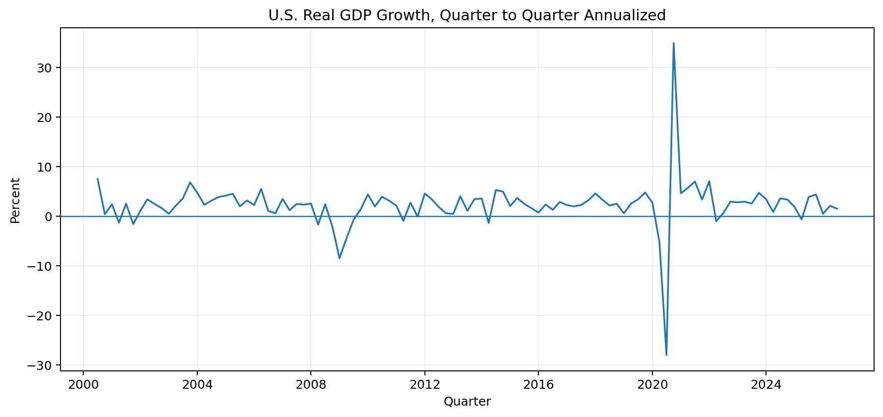
Create Lagged Features Without Data Leakage
Lagged variables are the core of this GDP forecasting Python workflow. The forecast for a quarter can use earlier GDP growth and earlier indicator values, but it cannot use data from the quarter being predicted unless the task is explicitly a nowcast.
The Ridge model uses four lags of GDP growth and one lag each of industrial production growth, real private investment growth, PCE inflation, and real government spending growth. The scaler is fitted inside a pipeline using training data only.
This design is conservative. It gives up some very recent information, but it makes the timing easy to explain and protects the backtest from look ahead bias.
Use a Time Ordered Train and Test Split
Random shuffling is wrong for a GDP forecasting Python task. A forecast made in 2023 should not learn from 2025 before it predicts 2023.
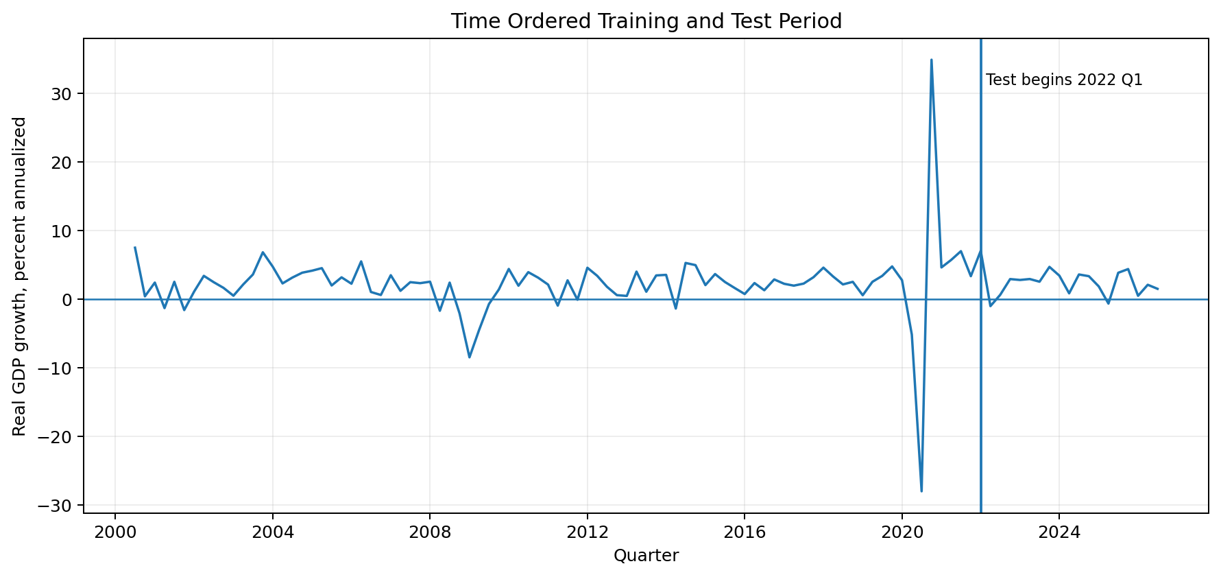
The worked example uses expanding rolling origin evaluation from 2022 Q1 through 2026 Q2. At each step, the model is fitted on all earlier observations, predicts the next quarter, then moves forward one quarter. This produces 18 out of sample forecasts.
The test period is recent enough to reflect the current economy, while the training history still includes the pandemic shock. That makes the exercise harder, but it also shows why GDP forecast uncertainty can become large.
Start With a Simple Baseline
A complex model has to beat something simple. The baseline in this tutorial assumes the next quarter will grow at the same annualized rate as the previous quarter.
That rule has no tuning and almost no explanation cost. If a more advanced model cannot improve on it, the extra complexity has not earned its place.
Model 1: Four Lag Autoregression
The autoregression uses the last four quarterly GDP growth observations, plus a constant and a time trend. It asks whether recent GDP growth contains enough information to improve on the persistence benchmark.
In the recent rolling test, this model produced the lowest MAE and RMSE. That does not prove it will remain the best model. It only means it performed best on the evaluation period used here.
Model 2: Ridge Regression With Lagged Indicators
The Ridge model adds lagged economic indicators to lagged GDP growth. Ridge regression is useful when predictors can move together because it shrinks coefficients instead of allowing unstable estimates to grow too large.
The model is placed in a scikit learn pipeline with StandardScaler. The scaler is refitted at every forecast origin using training data only. This detail matters because fitting a scaler on the full dataset leaks information from the future.
Rolling origin evaluation code
test_start = "2022-01-01"
predictions = []

for forecast_date in model_data.loc[test_start:].index:
    train = model_data.loc[
        model_data.index < forecast_date
    ]

    ar = AutoReg(
        train["gdp_growth"],
        lags=4,
        trend="ct",
        old_names=False
    ).fit()

    ar_pred = ar.predict(
        start=len(train),
        end=len(train)
    ).iloc[0]

    ridge = Pipeline([
        ("scale", StandardScaler()),
        ("model", Ridge(alpha=10.0))
    ])

    ridge.fit(
        train[feature_cols],
        train["gdp_growth"]
    )

    ridge_pred = ridge.predict(
        model_data.loc[[forecast_date], feature_cols]
    )[0]

    predictions.append({
        "date": forecast_date,
        "actual": model_data.loc[
            forecast_date,
            "gdp_growth"
        ],
        "autoreg": ar_pred,
        "ridge": ridge_pred
    })
Compare Forecast Accuracy
MAE measures the average absolute forecast error. RMSE also measures error, but it gives more weight to large misses. Lower values are better for both metrics.
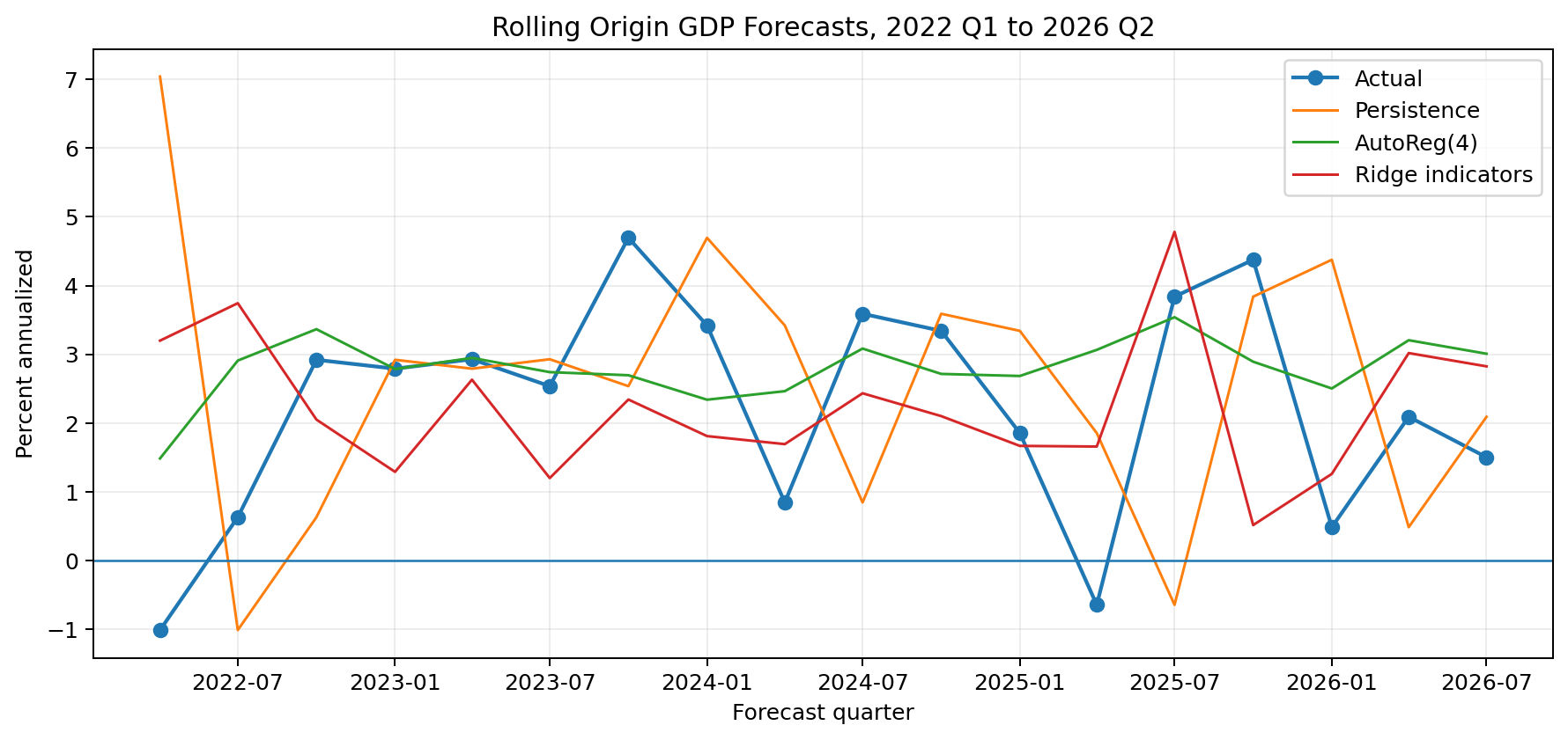
From 2022 Q1 through 2026 Q2, the four lag autoregression had an MAE of about 1.24 percentage points and an RMSE of about 1.57. The Ridge model had an MAE of about 1.60 and an RMSE of about 1.95. The persistence benchmark had an MAE of about 2.04 and an RMSE of about 2.79.
The autoregression also correctly identified whether growth would speed up or slow down from the prior quarter in about 83 percent of the test observations. Directional accuracy is only a secondary check, but it helps readers see a different side of forecast performance.
| Model | Horizon | Features | MAE | RMSE | Direction | Notes |
|---|---|---|---|---|---|---|
| Persistence | 1 quarter | Previous GDP growth | 2.04 | 2.79 | Not used | Simple benchmark |
| AutoReg(4) | 1 quarter | Four GDP growth lags plus trend | 1.24 | 1.57 | 83.3% | Best recent MAE and RMSE |
| Ridge indicators | 1 quarter | GDP lags plus lagged quarterly indicators | 1.60 | 1.95 | 77.8% | Regularized multivariate model |
Plot the Forecasts, Not Just the Scores
A model comparison table can hide when errors happened. The forecast chart shows that no model tracks every quarter perfectly. The visual check is especially important around turning points, when the economy can change faster than a simple time series rule.
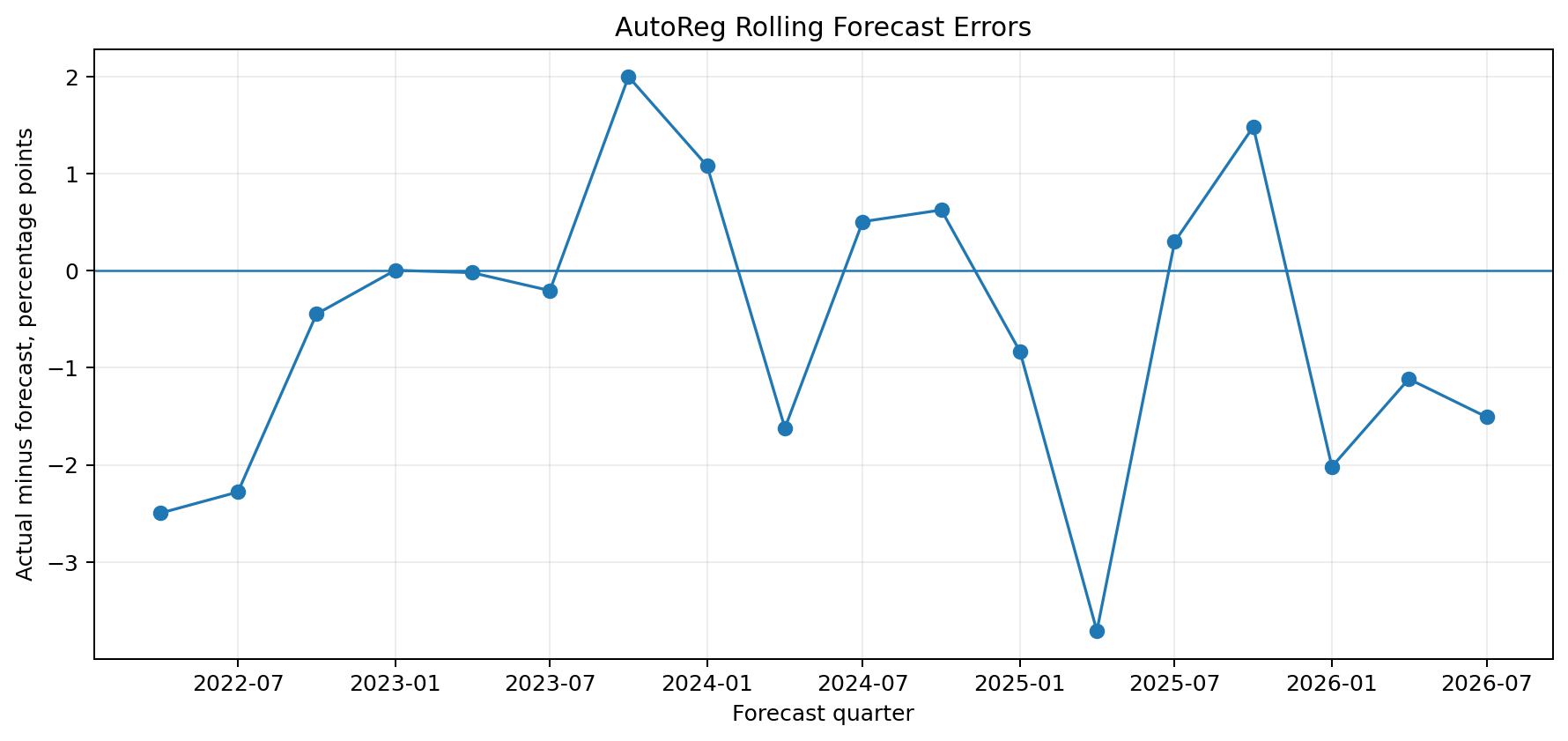
Residuals should also be inspected. A residual is actual growth minus forecast growth. Large or persistent residual patterns can show that the model is missing an important part of the data generating process.
Animate the Rolling Forecast Origins
The interactive animation is titled How the U.S. GDP Forecast Changes at Each Forecast Origin. Each frame shows the GDP growth history available at that stage, the one quarter ahead AutoReg forecast, the actual result after it became known, and the forecast error.
The purpose of the animation is educational. A normal static line can make a forecast look as if it was produced with knowledge of the future. Moving through forecast origins shows what the model knew at each step.
How the U.S. GDP Forecast Changes at Each Forecast Origin
Press Play to move through the rolling test. Hover over the forecast marker to see the predicted value, actual value, and error.
Forecast U.S. GDP Growth for 2026 Q3
After the evaluation, the selected four lag autoregression was refitted through 2026 Q2. Its tutorial forecast for 2026 Q3 is 3.0 percent annualized real GDP growth. The persistence benchmark gives 1.5 percent, while the Ridge indicator model gives 2.5 percent.
The AutoReg model also produces a wide 80 percent model based interval, from about -3.3 percent to 9.4 percent. That range is a reminder that quarterly GDP is difficult to predict. The model was estimated on a history that includes extreme pandemic movements, which increases estimated uncertainty.
This is a tutorial model forecast, not an official BEA forecast, a Federal Reserve forecast, or a market consensus. It should be used to understand the forecasting workflow rather than as a trading or policy signal.
| Forecast quarter | Point forecast | Lower 80% | Upper 80% | Model | Data vintage |
|---|---|---|---|---|---|
| 2026 Q3 | 3.04% | -3.27% | 9.36% | AutoReg(4) | Data through 2026 Q2, accessed Aug 20 2026 |
final_model = AutoReg(
    model_data["gdp_growth"],
    lags=4,
    trend="ct",
    old_names=False
).fit()

forecast = final_model.get_prediction(
    start=len(model_data),
    end=len(model_data)
)

forecast_table = forecast.summary_frame(alpha=0.20)
print(forecast_table)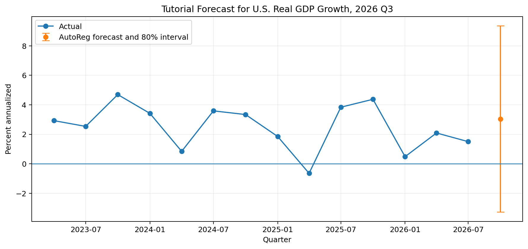
Forecast Uncertainty and Data Revisions Matter
GDP data are revised. BEA publishes an advance estimate, later estimates, and periodic annual updates. FRED normally shows the latest revised history. If you train a historical model on today's revised series, the model may see values that forecasters did not know at the time.
For a GDP forecasting Python backtest, that problem is called revision bias or vintage bias. For a serious real time backtest, use ALFRED or another vintage data source so every historical forecast uses the data available on that date.
The current tutorial uses the latest revised series because it is easier for readers to reproduce. That choice is clearly stated as a limitation.
Common GDP Forecasting Mistakes
The most common mistake is forecasting the GDP level and then judging the model mainly by a high R squared value. A smooth upward level can create impressive looking scores without a useful growth forecast.
Other mistakes include random train and test splits, fitting a scaler on the whole dataset, using revised values as if they were known in real time, mixing monthly and quarterly data without a timing rule, and using a monthly value from the forecast quarter before it was released.
Another mistake is reporting one point forecast without uncertainty. Even a well tested model can miss badly during a shock or turning point. Forecasts are estimates, not promises.
Conclusion
A useful GDP forecasting Python project is mostly about discipline. Define the growth target clearly, respect the order of time, compare every model with a simple benchmark, and judge performance on quarters the model did not train on.
In this worked example, the four lag autoregression produced the best recent rolling test scores and a tutorial forecast of about 3.0 percent annualized growth for 2026 Q3. The wide interval matters as much as the point estimate. GDP revisions, shocks, and changing relationships can quickly make a neat model uncertain.
The next step is to rerun the workflow after each BEA GDP release. For a more serious forecasting system, replace revised historical data with ALFRED vintages, add carefully timed monthly indicators, and compare the results with the same rolling evaluation.
Frequently Asked Questions
How do I forecast GDP in Python?
Start with real GDP, convert the level into a growth rate, create lagged features, keep the data in time order, fit a benchmark and one or more forecasting models, then test them with rolling one quarter ahead predictions before making the next forecast.
What is the best Python model for GDP forecasting?
There is no single best model for every period. A simple autoregression can be hard to beat, while indicator models can help when leading data add useful information. Choose the model with out of sample evidence, not in sample fit alone.
Which FRED series should I use for U.S. real GDP?
GDPC1 is the main FRED series for real U.S. GDP. It is sourced from BEA, reported quarterly, and measured in billions of chained 2017 dollars at a seasonally adjusted annual rate.
How do I calculate quarterly GDP growth?
One common method is 100 times the quantity of current GDP divided by previous GDP, raised to the fourth power, minus one. This converts a quarter to quarter change into an annualized rate.
Can ARIMA forecast GDP?
Yes. ARIMA and related autoregressive models are common starting points for GDP growth. They are useful benchmarks because they use the history of the target itself. Their performance should still be tested on future periods.
Which economic indicators can help forecast GDP?
Industrial production, employment, unemployment, investment, inflation, interest rates, sales, and income can all add information. The key is to use only data that would have been available at the forecast date.
How should I split time series data for GDP forecasting?
Keep observations in time order. Train on the past and test on later quarters. Rolling origin or walk forward evaluation is better than a random split because it copies the way a forecast is made in real life.
Why do GDP data revisions matter?
BEA revises GDP as more complete source data arrive. A backtest that uses today's revised history can be too optimistic because earlier forecasters did not know those revised values. ALFRED can help with real time vintage analysis.
Suggested Internal Links
- FRED API in Python: Download and Analyze U.S. Economic Data
- Analyze the U.S. Unemployment Rate in Python
- U.S. Inflation Data Analysis With Python
Methodology and Limitations
The worked dataset uses quarterly observations from 2000 Q1 through 2026 Q2. The target is quarter to quarter real GDP growth at an annualized rate calculated from FRED series GDPC1.
The rolling model comparison covers 2022 Q1 through 2026 Q2. The persistence benchmark repeats the prior quarter. AutoReg uses four GDP growth lags with a constant and time trend. Ridge uses four GDP growth lags plus one quarter lagged growth in industrial production, real private investment, the PCE price index, and real government consumption and investment.
All indicator features are lagged by one quarter in the Ridge model. The StandardScaler is fitted inside the training pipeline. This avoids using information from the forecast quarter.
The model uses the latest revised historical series available on August 20, 2026. It is not a true real time vintage backtest. Historical revisions can make backtest results look better than a forecast made with the data available at the time.
The final 2026 Q3 value is a tutorial model forecast. It is not an official BEA forecast and should not be used as a guarantee of future growth.
Official Sources
- BEA GDP Advance Estimate, Second Quarter 2026
- FRED GDPC1, Real Gross Domestic Product
- FRED IPB50001SQ, Industrial Production
- FRED GPDIC1, Real Gross Private Domestic Investment
- FRED PCECTPI, PCE Price Index
- FRED GCEC1, Real Government Consumption and Investment
- FRED API documentation
- FRED real time periods and ALFRED guidance
Downloads
Files attached to this article for your reference.