
Logistic Regression Explained: How It Works in ML
Logistic regression is a supervised machine learning algorithm that estimates the probability of a categorical outcome. It is most often used for binary classification, such as spam versus legitimate email, fraud versus…
Logistic Regression: How It Works in Machine Learning
Logistic regression is a supervised machine learning algorithm that estimates the probability of a categorical outcome. It is most often used for binary classification, such as spam versus legitimate email, fraud versus valid activity, or customer churn versus retention.
The model does not jump directly from input data to a yes-or-no answer. It first produces a probability between 0 and 1. A decision threshold then converts that probability into a class label. This distinction is central to using the method well: the model estimates likelihood, while the threshold represents the operational decision.
What Is Logistic Regression in Machine Learning?
Despite its name, logistic regression is used primarily as a classification algorithm in machine learning. It is a linear model because it assumes that the log odds of the outcome can be written as a linear combination of the input features. In the binary case, the target normally has two values, such as 0 and 1.[1]
Consider a bank estimating whether an applicant will default. Income, repayment history, debt level, and credit utilization can become input features. The logistic regression model may return a default probability of 0.72. A separate business rule then determines whether that score leads to approval, rejection, or manual review.
This probability-first design is why the method is useful beyond simple class prediction. It can rank cases by risk, support different actions at different thresholds, and show how each modeled feature is associated with the outcome.
Why Logistic Regression Still Matters in Modern Machine Learning
Newer machine learning methods can model more complicated patterns, but greater complexity does not automatically produce a better decision system. Logistic regression remains useful because it is fast, comparatively transparent, and easy to test as a baseline.
Its coefficients can be converted into odds ratios, its predicted probabilities can be evaluated for calibration, and regularization can control unstable or overly large coefficients. Scikit-learn supports regularized binary and multinomial logistic models with multiple optimization solvers.[2][4]
In regulated or high-impact settings, interpretability can be as important as raw predictive performance. A credit team, healthcare analyst, or SaaS retention manager may need to explain which variables influenced a score, how the probability was translated into action, and what types of error the system accepts.
The contrarian but practical view is that logistic regression is not merely a beginner algorithm to replace later. If it performs close to a more complex model under realistic validation, its lower deployment and maintenance burden may make it the better production choice.
How Logistic Regression Works Step by Step
The linear score combines features, weights, and an intercept
The calculation begins with a linear score:
Here, X contains the input features, w contains the learned coefficients or weights, and b is the intercept, sometimes called the bias term. The score z can take any value from negative infinity to positive infinity, so it cannot be interpreted directly as a probability.
The sigmoid function converts the score into probability
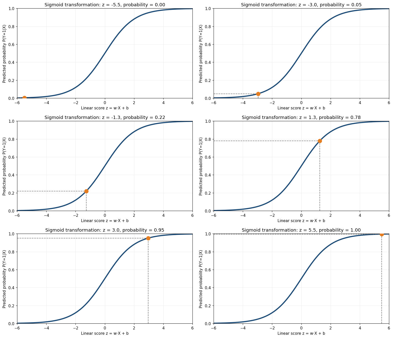
The sigmoid, also called the logistic function, transforms the unrestricted score into a number between 0 and 1:
As z becomes strongly positive, the probability approaches 1. As z becomes strongly negative, the probability approaches 0. A score of zero produces a probability of 0.5. The transformation creates the familiar S-shaped sigmoid curve.
A probability threshold creates the final class
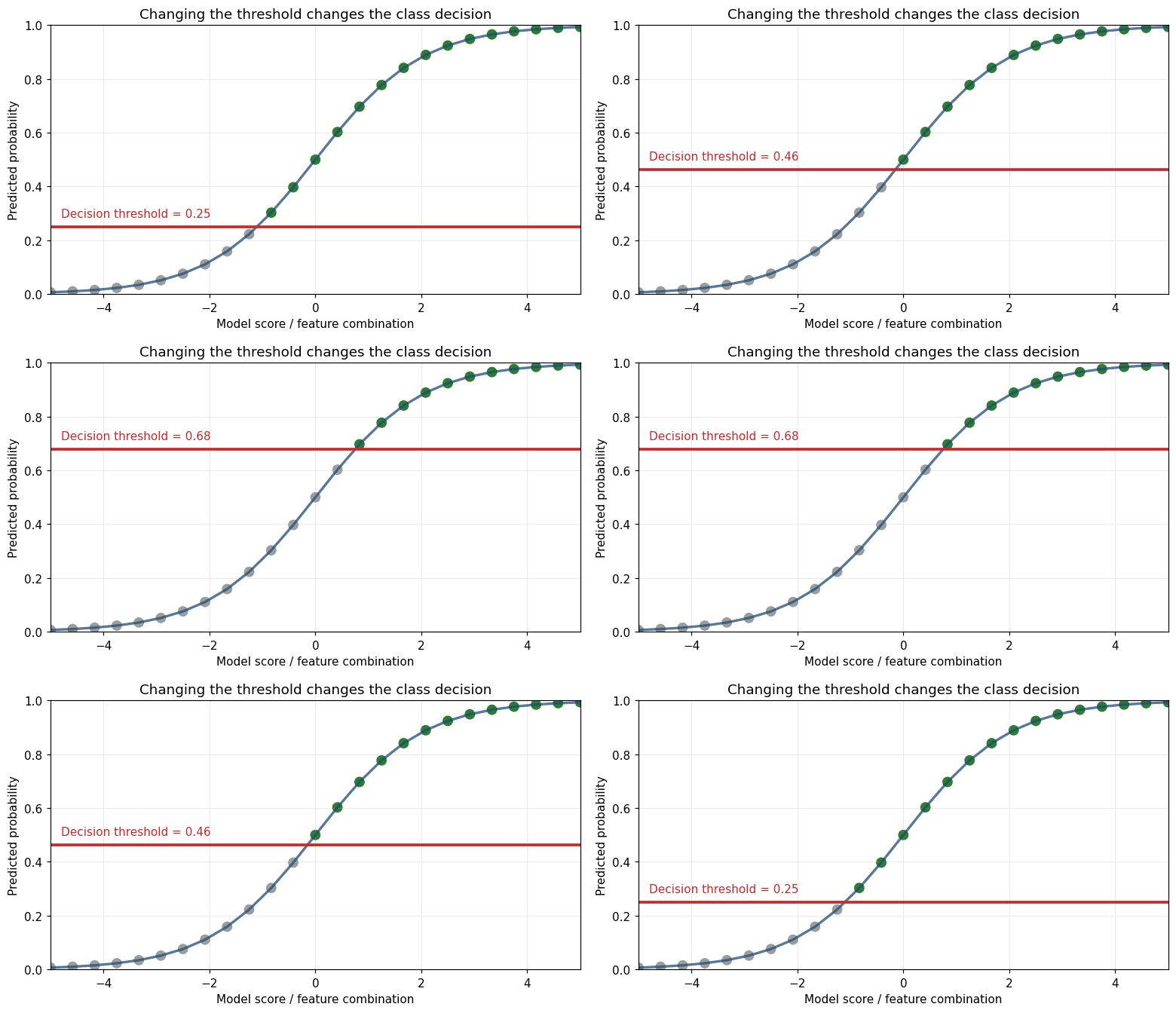
A binary classifier commonly uses 0.5 as the default threshold, but that cutoff is not a mathematical requirement. Scikit-learn separates probability estimation from the decision rule and provides tools for selecting a threshold that better matches the chosen metric or operational cost.[1][3]
At a threshold of 0.5, a predicted probability of 0.82 becomes Class 1 and a probability of 0.23 becomes Class 0. Raising the threshold usually reduces the number of positive predictions, while lowering it usually identifies more potential positives.
This is where theory meets actual use. In medical screening, missing a true case may be more harmful than investigating an extra false alarm, so recall may receive greater weight. In fraud review, an organization with limited investigators may require higher precision before sending a transaction to manual review.
Probability, Odds, and Log Odds Explained
Probability describes the chance that an event occurs. Odds compare the probability of the event with the probability that it does not occur:
A churn probability of 0.75 corresponds to odds of 0.75 divided by 0.25, or 3. The modeled odds of churn are therefore three to one.
Probabilities are restricted to the interval from 0 to 1, while odds range from 0 to positive infinity. Logistic regression takes the natural logarithm of the odds to create the logit, or log odds:
The model is linear in the log odds, not in the raw probability. This is an important semantic distinction. It does not assume that adding one year of age or one support ticket causes the probability to rise by the same amount everywhere on the sigmoid curve.
How to Interpret Logistic Regression Coefficients
A coefficient represents the expected change in log odds associated with a one-unit increase in a feature, while the other included features are held constant. A positive coefficient raises the modeled log odds of the positive class; a negative coefficient lowers them.
Exponentiating a coefficient converts it into an odds ratio:
If a coefficient is approximately 0.693, its odds ratio is about 2. A one-unit increase in that feature multiplies the modeled odds by roughly two, assuming the rest of the model remains unchanged. A coefficient of zero gives an odds ratio of one, indicating no change in the odds.
Coefficient size should not be compared blindly across features measured on different scales. A one-unit increase in annual income is not equivalent to a one-unit increase in the number of complaints. Standardization or domain-relevant units make interpretation clearer.
Coefficients are associations within the fitted model. They do not establish that changing a feature will cause the outcome to change. Causal claims require an appropriate research design and stronger assumptions than ordinary predictive modelling provides.
How Maximum Likelihood Estimation Trains the Model
Classical binary logistic regression estimates its coefficients through maximum likelihood. The method chooses parameter values that make the observed outcomes as probable as possible under the model. Statsmodels’ Logit implementation fits the model through maximum likelihood.[7]
When the observed class is 1, the likelihood rewards a high predicted probability. When the observed class is 0, it rewards a low predicted probability. Because multiplying many probabilities can create extremely small values, software normally works with the log-likelihood, which converts the product into a sum.
Machine learning libraries often optimize a penalized version of this objective. Scikit-learn applies regularization by default, so its LogisticRegression estimator is not identical to an unpenalized statistical logit model. Regularization can improve numerical stability and reduce overfitting, but it also shrinks coefficient estimates.[1][2]
Gradient-based solvers iteratively adjust the coefficients to reduce log loss or, equivalently in the unpenalized case, increase the log-likelihood. The best solver depends on sample size, feature count, sparsity, multiclass requirements, and the selected form of regularization.
Types of Logistic Regression
Binary logistic regression
Binary logistic regression handles two outcomes. Typical examples include fraud versus legitimate activity, churn versus retention, default versus repayment, and a positive versus negative test result.
Multinomial logistic regression
Multinomial logistic regression handles three or more classes without a natural order. Instead of one sigmoid output, the model can use the softmax function to estimate a probability for each class, with all class probabilities summing to one. Current scikit-learn solvers support multinomial loss except where the documentation states otherwise.[1][2]
Ordinal logistic regression
Ordinal logistic regression is designed for ordered categories such as poor, fair, good, and excellent. It preserves information about the ranking of the outcomes rather than treating every category as unrelated. Statsmodels provides an OrderedModel that supports logit and probit distributions.[8]
Logistic Regression vs Linear Regression
| Feature | Linear Regression | Logistic Regression |
|---|---|---|
| Purpose | Predict a continuous numerical value | Estimate probabilities for categorical outcomes |
| Typical output | Price, demand, age, or temperature | Probability of a class and an optional class label |
| Output range | Unbounded | Between 0 and 1 after the logistic transformation |
| Model shape | Linear prediction | Sigmoid-transformed linear score |
| Common estimation | Ordinary least squares | Maximum likelihood or penalized log loss |
| Example | Predicting a house price | Predicting whether a customer will churn |
The naming can be confusing because both methods contain a linear component. Linear regression predicts a numerical value directly. Logistic regression predicts log odds and converts them into a class probability. The latter is therefore used as a classifier in standard machine learning terminology.
Assumptions and Data Requirements
The target must match the selected model type: binary for ordinary binary logistic regression, unordered multiclass for a multinomial model, or ordered categories for an ordinal model.
Observations should provide independent information unless the model explicitly accounts for grouping, repeated measurements, or time dependence. Allowing records from the same patient, customer, household, or device to appear in both training and test sets can exaggerate performance.
The key functional assumption is linearity between the supplied predictors and the log odds. Logistic regression does not require a straight-line relationship between a feature and the raw probability. Curved relationships may require transformations, splines, polynomial terms, or meaningful interactions.
Strong multicollinearity can make coefficients unstable, and near-perfect separation can drive estimates toward extreme values. Regularization often helps, but it does not repair incorrect target definitions, leakage, poor sampling, or missing causal structure.
There is no universal minimum sample size. The amount of data required depends on the number of predictors, outcome frequency, class imbalance, feature quality, regularization, and the level of uncertainty the application can tolerate.
A Practical Logistic Regression Workflow
Define the outcome before selecting the algorithm
Specify the positive class, the prediction window, and the moment at which the prediction will be made. “Customer churn” could mean cancellation within 30 days, 90 days, or one year. Each definition produces a different dataset and a different decision problem.
Create a validation design that resembles future use
Split the data before learning preprocessing steps. Scaling, imputation, feature selection, and encoding should be fitted using training data only. Scikit-learn recommends pipelines as a practical way to prevent information from the test set leaking into model training.[5]
Time-based problems often require chronological validation. Repeated customers, patients, or devices may require group-aware splitting. A random split is convenient, but it is not always realistic.
Prepare and encode the features
Categorical variables normally need encoding, missing values need an explicit strategy, and numerical features may need scaling. Feature engineering should represent relationships that the basic linear log-odds structure cannot discover automatically.
Train, tune, and preserve the final test set
Use cross-validation or a separate validation set to choose regularization strength and other hyperparameters. Do not repeatedly inspect the final test set while tuning the model, because this quietly turns the test data into part of the development process.
Evaluate probabilities and decisions separately
Discrimination asks whether the model ranks positive cases above negative cases. Calibration asks whether predicted probabilities match observed frequencies. Scikit-learn’s calibration guidance uses reliability diagrams to compare predicted probabilities with actual outcome rates.[4]
A model can rank cases well while producing probabilities that are consistently too high or too low. This matters when the probability itself drives pricing, staffing, treatment, or financial reserves.
Evaluation Metrics for Logistic Regression
Accuracy is the share of correct classifications, but it can hide complete failure on a rare class. If only 1 percent of transactions are fraudulent, predicting every transaction as legitimate produces 99 percent accuracy and detects no fraud.
Precision measures the proportion of predicted positives that are correct. Recall measures the proportion of actual positives that the model identifies. The F1 score combines precision and recall through their harmonic mean.
ROC-AUC summarizes ranking performance across thresholds. Precision-recall analysis is often more revealing when the positive class is rare because it focuses on the quality and coverage of positive predictions. Log loss evaluates probability estimates and penalizes confident mistakes more heavily.[6]
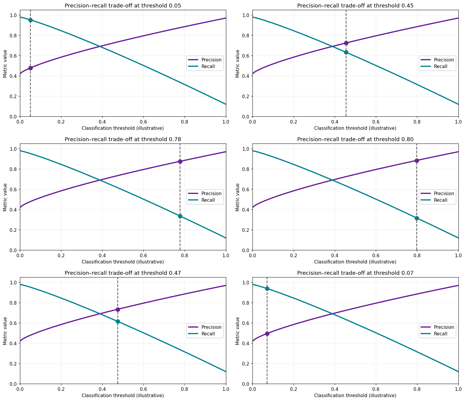
The correct metric depends on the real cost of errors. A metric should represent the decision, not merely be convenient to calculate.
Use Our Logistic Regression Calculator
A logistic regression calculator can make the mathematics easier to check without writing code. Enter the intercept, feature values, and coefficients to calculate the linear score, predicted probability, odds, and class at a selected threshold.
Calculate a probability from your own coefficients and feature values.
Open the Logistic Regression CalculatorPublisher note: replace this placeholder URL with your calculator’s final website address before publishing.
The calculator is most useful for learning how individual inputs change a prediction, checking a coefficient interpretation, or demonstrating why the same probability can lead to different decisions at different thresholds. It should not replace model validation, calibration testing, or a complete data pipeline.
Logistic Regression in Python with Scikit-Learn
The following logistic regression example uses the breast cancer dataset included with scikit-learn. A pipeline standardizes the features and fits the classifier without leaking test-set information into preprocessing.
from sklearn.datasets import load_breast_cancer
from sklearn.linear_model import LogisticRegression
from sklearn.metrics import classification_report, confusion_matrix, roc_auc_score
from sklearn.model_selection import train_test_split
from sklearn.pipeline import make_pipeline
from sklearn.preprocessing import StandardScaler

X, y = load_breast_cancer(return_X_y=True)

X_train, X_test, y_train, y_test = train_test_split(
    X, y,
    test_size=0.20,
    random_state=42,
    stratify=y,
)

model = make_pipeline(
    StandardScaler(),
    LogisticRegression(max_iter=2000),
)

model.fit(X_train, y_train)
positive_probability = model.predict_proba(X_test)[:, 1]

threshold = 0.50
predictions = (positive_probability >= threshold).astype(int)

print(confusion_matrix(y_test, predictions))
print(classification_report(y_test, predictions))
print("ROC-AUC:", roc_auc_score(y_test, positive_probability))
The example is a starting point, not a production recipe. A real project should validate the split strategy, tune regularization, examine class definitions, evaluate calibration, and choose a threshold based on the consequences of false positives and false negatives.[2][3][4][5]
Real-World Applications
Fraud detection and risk scoring
A fraud model can estimate the probability that a transaction is suspicious using amount, location changes, account age, device signals, and behavioral history. The threshold determines whether the transaction is approved, challenged, blocked, or sent for review.
Healthcare prediction
Healthcare researchers can use the method to estimate the probability of an outcome from patient characteristics. The model still requires clinical validation, representative data, calibration, and governance. A predicted probability should not be presented as a diagnosis without the necessary medical evidence and oversight.
Customer churn and SaaS retention
A SaaS business can estimate which accounts are likely to cancel by combining contract age, product usage, payment behavior, support activity, and engagement trends. The score can prioritize retention outreach, but using post-cancellation information or future activity would create leakage.
Marketing, lead conversion, and credit risk
Marketing teams can estimate response or purchase probability, while financial institutions can model default risk or application outcomes. In each case, the operational value depends on data quality, fair and lawful use, calibration, and a threshold that reflects the true cost of errors.
Advantages and Limitations of Logistic Regression
The main advantages are speed, interpretability, efficient probability estimation, support for regularization, and strong compatibility with sparse or tabular data. It is often easier to deploy and monitor than a large ensemble or neural network.
The main limitation is structural. A basic logistic regression algorithm creates a linear decision boundary in the supplied feature space. It will not automatically discover complicated thresholds, interactions, or nonlinear patterns. Those relationships must be represented through feature engineering or handled by a more flexible model.
Interpretability also has boundaries. Correlated predictors can make individual coefficients unstable, regularization changes their magnitude, and a transparent equation does not guarantee that the dataset or decision process is fair.
Maintenance remains necessary. Shifts in customer behavior, fraud tactics, clinical practice, pricing, or data collection can reduce calibration and predictive performance after deployment.
Common Mistakes That Reduce Model Performance
The most common mistake is evaluating only accuracy. Other recurring problems include treating 0.5 as automatically optimal, selecting a threshold on the final test set, allowing data leakage, ignoring time or group structure, and interpreting association as causation.
Another mistake is assuming that scaling is always optional. Scaling may not change the mathematical meaning of an unpenalized model, but it can affect optimization, regularization, and the comparability of coefficient magnitudes.
Feature engineering can also fail in two opposite ways. Too little feature design leaves important nonlinear relationships unmodeled; too many arbitrary interactions increase variance and make the system difficult to maintain. Domain knowledge should guide which transformations are worth testing.
Logistic Regression vs Other Classification Algorithms
Decision trees learn rule-based splits and can capture nonlinear relationships without manually adding transformations. Random forests combine many trees and usually model complex interactions more easily, but the resulting decision process is less compact than one logistic equation.
Support vector machines can work well in high-dimensional spaces and can use kernels for nonlinear boundaries. Their probability estimates are less direct and may require an additional calibration step.
The most defensible comparison is empirical. Train the alternatives on the same data, use the same validation design, and compare discrimination, calibration, interpretability, latency, fairness checks, and maintenance cost. A small improvement in ROC-AUC may not justify a much more expensive system.
When Should You Use Logistic Regression?
Use logistic regression when the target is categorical, probability estimates matter, and the relationship can be represented adequately through linear terms, transformations, and a manageable number of interactions. It is especially suitable when stakeholders need an understandable baseline or when deployment resources are limited.
It is also a strong first model for tabular classification. A more complex algorithm should demonstrate a meaningful and repeatable improvement under realistic validation before replacing it.
When Should You Avoid It?
A basic logistic regression model may be a poor fit when the data contains highly complex nonlinear structures that cannot be represented through reasonable feature engineering. Raw image, audio, and video tasks usually require representation-learning methods before classification.
Avoid relying on an ordinary fit when classes are nearly perfectly separated, predictors are severely collinear, the positive outcome is too rare for stable estimation, or future data differs substantially from the training population. These conditions require redesign, stronger regularization, more data, a different model, or a different decision process.
Why Logistic Regression Still Matters in 2026
Logistic regression remains actively supported in current machine learning and statistical software. Scikit-learn provides binary and multinomial classification, several regularization choices, multiple solvers, probability outputs, model evaluation tools, calibration workflows, and threshold tuning. Statsmodels continues to support likelihood-based binary and ordered models.[1][2][3][4][7][8]
Its continued relevance is not based on novelty. It comes from the need for decision systems that can be explained, validated, monitored, and operated at reasonable cost.
Generative AI tools and AutoML platforms may help write code or compare models, but they do not remove the need to define the target, prevent leakage, validate on realistic data, select an appropriate metric, and understand the cost of errors. Those choices remain human and domain-specific.
Frequently Asked Questions
What is logistic regression used for?
It is used to estimate the probability of a categorical outcome. Common applications include fraud screening, churn prediction, credit risk, medical research, spam classification, and lead conversion modelling.
Is logistic regression classification or regression?
In machine learning, it is generally classified as a classification algorithm. The name refers to modeling the log odds through a linear equation rather than predicting a continuous target in the way linear regression does.[1]
Why is the sigmoid function used?
The sigmoid converts any real-valued linear score into a number between 0 and 1, allowing the result to be interpreted as the probability of the positive class.
Does logistic regression require a large dataset?
Not always. Required sample size depends on predictor count, class balance, outcome rarity, feature quality, regularization, and the level of reliability the application needs. A large total sample can still be insufficient when the positive class is extremely rare.
How accurate is logistic regression?
There is no universal accuracy level. Performance depends on the problem, target definition, data quality, feature design, validation method, and comparison metric. The method should be evaluated on unseen data that resembles its intended use.
What is the biggest limitation?
The basic model assumes a linear relationship between the supplied predictors and the log odds. It can miss complex nonlinear patterns and interactions unless those relationships are engineered into the feature set.
Is logistic regression still used in artificial intelligence?
Yes. It remains useful as an interpretable classifier, a probability model, a baseline for more complex systems, and a final classification layer when another method has already created informative features.
Conclusion: Turning Logistic Regression Probabilities into Better Decisions
Logistic regression is most useful when it is treated as a complete decision framework rather than only an S-shaped formula. The model combines features into log odds, converts those log odds into probability, and leaves the final action to a threshold chosen around real costs and priorities.
Start with a clear target, a realistic validation design, leakage-safe preprocessing, and metrics that reflect the application. Keep logistic regression when it delivers reliable, calibrated results with an acceptable error trade-off. Move to a more complex method only when the improvement is meaningful enough to justify the extra effort, opacity, and maintenance.
The practical next step is to test the model on representative data, inspect its coefficients and probability calibration, and use the logistic regression calculator to verify how specific inputs and thresholds affect the final prediction.
You May Also Like Spearman Correlation
References
[1] Scikit-learn, “Logistic regression” in Linear Models.
[2] Scikit-learn, LogisticRegression API documentation.
[3] Scikit-learn, Decision threshold tuning.
[4] Scikit-learn, Probability calibration.
[5] Scikit-learn, Common pitfalls and data leakage.
[6] Scikit-learn, Metrics and scoring.
Try it in DataClue
Ready to run Logistic Regression?
Model the probability of a binary outcome based on one or more predictor variables.
Run Logistic Regression